Introduction

介绍

First encountering a new dataset can sometimes feel overwhelming. You might be presented with hundreds or thousands of features without even a description to go by. Where do you even begin?

第一次遇到新的数据集有时会让人感到不知所措。 您可能会看到成百上千个特征，甚至没有任何说明。 你从哪里开始呢？

A great first step is to construct a ranking with a feature utility metric, a function measuring associations between a feature and the target. Then you can choose a smaller set of the most useful features to develop initially and have more confidence that your time will be well spent.

第一步是使用 功能效用指标 构建排名，这是一个衡量功能与目标之间关联的函数。 然后，您可以选择一小部分最有用的功能进行最初开发，可以肯定您的时间不会被浪费。

The metric we'll use is called "mutual information". Mutual information is a lot like correlation in that it measures a relationship between two quantities. The advantage of mutual information is that it can detect any kind of relationship, while correlation only detects linear relationships.

我们将使用的指标称为互信息。 互信息很像相关性，因为它衡量两个量之间的关系。 互信息的优点是它可以检测任何类型的关系，而相关性只能检测线性关系。

Mutual information is a great general-purpose metric and especially useful at the start of feature development when you might not know what model you'd like to use yet. It is:

互信息是一个很好的通用指标，在功能开发开始时（当您可能还不知道要使用什么模型时）特别有用。 这是：

• easy to use and interpret,
• 易于使用和解释，
• computationally efficient,
• 计算效率高，
• theoretically well-founded,
• 理论上有充分依据，
• resistant to overfitting, and,
• 抵抗过度拟合，并且，
• able to detect any kind of relationship
• 能够检测任何类型的关系

Mutual Information and What it Measures

互信息及其测量内容

Mutual information describes relationships in terms of uncertainty. The mutual information (MI) between two quantities is a measure of the extent to which knowledge of one quantity reduces uncertainty about the other. If you knew the value of a feature, how much more confident would you be about the target?

互信息用不确定性来描述关系。 两个量之间的互信息（MI）是衡量一个量信息的减少导致另一个量的不确定性程度增加的度量。 如果您知道某个特征的价值，您对目标的信心会有多大？

Here's an example from the Ames Housing data. The figure shows the relationship between the exterior quality of a house and the price it sold for. Each point represents a house.

以下是艾姆斯住房数据的示例。 该图显示了房屋的外部质量与其售价之间的关系。 每个点代表一座房子。

Knowing the exterior quality of a house reduces uncertainty about its sale price.
了解房屋的外部质量可以减少其售价的不确定性。

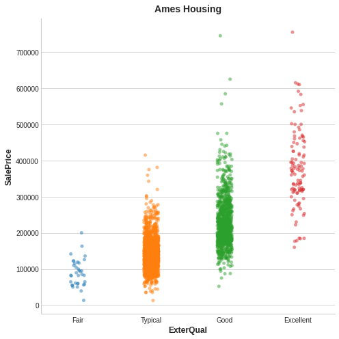
From the figure, we can see that knowing the value of ExterQual should make you more certain about the corresponding SalePrice -- each category of ExterQual tends to concentrate SalePrice to within a certain range. The mutual information that ExterQual has with SalePrice is the average reduction of uncertainty in SalePrice taken over the four values of ExterQual. Since Fair occurs less often than Typical, for instance, Fair gets less weight in the MI score.

从图中我们可以看出，知道了 ExterQual 的值应该可以让您更加确定 SalePrice —— 每个ExterQual的类别都倾向于将 SalePrice 集中在一定的范围内。 ExterQual与SalePrice的互信息是SalePrice对ExterQual的四个值的不确定性的平均减少量。 例如，由于一般出现的频率低于典型，因此一般在 MI 分数中的权重较小。

(Technical note: What we're calling uncertainty is measured using a quantity from information theory known as "entropy". The entropy of a variable means roughly: "how many yes-or-no questions you would need to describe an occurance of that variable, on average." The more questions you have to ask, the more uncertain you must be about the variable. Mutual information is how many questions you expect the feature to answer about the target.)

（技术说明：我们所说的不确定性是使用信息论中称为熵的量来测量的。变量的熵大致意味着：您平均需要多少是或否的问题来描述变量的出现。您要问的问题越多，您对变量的不确定性就越大。互信息是您期望用多少关于特征的问题来回答目标的情况。）

Interpreting Mutual Information Scores

解释互信息得分

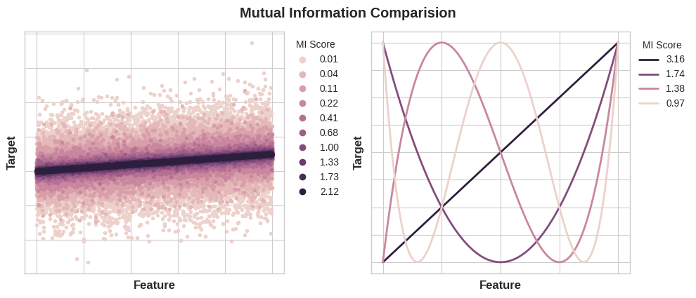
The least possible mutual information between quantities is 0.0. When MI is zero, the quantities are independent: neither can tell you anything about the other. Conversely, in theory there's no upper bound to what MI can be. In practice though values above 2.0 or so are uncommon. (Mutual information is a logarithmic quantity, so it increases very slowly.)

数量之间的最小可能互信息为 0.0。 当 MI 为零时，这些量是独立的：两者都无法告诉您有关对方的任何信息。 相反，理论上 MI 没有上限。 但实际上，高于 2.0 左右的值并不常见。 （互信息是一个对数量，因此增长非常缓慢。）

The next figure will give you an idea of how MI values correspond to the kind and degree of association a feature has with the target.

下图将让您了解 MI 值如何对应于特征与目标的关联类型和程度。

Left: Mutual information increases as the dependence between feature and target becomes tighter. Right: Mutual information can capture any kind of association (not just linear, like correlation.)
左：随着特征和目标之间的依赖性变得更加紧密，互信息也会增加。 右：互信息可以捕捉任何类型的关联（不仅仅是线性的，如相关性。）

Here are some things to remember when applying mutual information:

应用互信息时需要记住以下几点：

• MI can help you to understand the relative potential of a feature as a predictor of the target, considered by itself.
• MI 可以帮助您了解某个特征作为目标预测因子（单独考虑）的“相对潜力”。
• It's possible for a feature to be very informative when interacting with other features, but not so informative all alone. MI can't detect interactions between features. It is a univariate metric.
• 一个特征在与其他特征交互时可能会提供非常丰富的信息，但单独使用时可能不会提供如此多的信息。 MI 无法检测功能之间的交互 。 这是一个单变量指标。
• The actual usefulness of a feature depends on the model you use it with. A feature is only useful to the extent that its relationship with the target is one your model can learn. Just because a feature has a high MI score doesn't mean your model will be able to do anything with that information. You may need to transform the feature first to expose the association.
• 特征的 实际 有用性 取决于您使用它时的模型 。 一项特征仅在其与目标的关系是您的模型可以学习的范围内才有用。 仅仅因为某个特征具有高 MI 分数并不意味着您的模型能够利用该信息执行任何操作。 您可能需要首先转换特征才能展现关联性。

Example - 1985 Automobiles

示例 - 1985 年汽车

The Automobile dataset consists of 193 cars from the 1985 model year. The goal for this dataset is to predict a car's price (the target) from 23 of the car's features, such as make, body_style, and horsepower. In this example, we'll rank the features with mutual information and investigate the results by data visualization.

汽车 数据集包含 193 辆 1985 年车型的汽车。 该数据集的目标是根据汽车的 23 个特征（例如品牌、车身风格和马力）预测汽车的价格（目标）。 在此示例中，我们将利用互信息对特征进行排序，并通过数据可视化研究结果。

This hidden cell imports some libraries and loads the dataset.

该隐藏单元导入一些库并加载数据集。

import matplotlib.pyplot as plt
import numpy as np
import pandas as pd
import seaborn as sns

plt.style.use("seaborn-v0_8-whitegrid")

df = pd.read_csv("../00 datasets/ryanholbrook/fe-course-data/autos.csv")

df.head()

	symboling	make	fuel_type	aspiration	num_of_doors	body_style	drive_wheels	engine_location	wheel_base	length	...	engine_size	fuel_system	bore	stroke	compression_ratio	horsepower	peak_rpm	city_mpg	highway_mpg	price
0	3	alfa-romero	gas	std	2	convertible	rwd	front	88.6	168.8	...	130	mpfi	3.47	2.68	9	111	5000	21	27	13495
1	3	alfa-romero	gas	std	2	convertible	rwd	front	88.6	168.8	...	130	mpfi	3.47	2.68	9	111	5000	21	27	16500
2	1	alfa-romero	gas	std	2	hatchback	rwd	front	94.5	171.2	...	152	mpfi	2.68	3.47	9	154	5000	19	26	16500
3	2	audi	gas	std	4	sedan	fwd	front	99.8	176.6	...	109	mpfi	3.19	3.40	10	102	5500	24	30	13950
4	2	audi	gas	std	4	sedan	4wd	front	99.4	176.6	...	136	mpfi	3.19	3.40	8	115	5500	18	22	17450

5 rows × 25 columns

The scikit-learn algorithm for MI treats discrete features differently from continuous features. Consequently, you need to tell it which are which. As a rule of thumb, anything that must have a float dtype is not discrete. Categoricals (object or categorial dtype) can be treated as discrete by giving them a label encoding. (You can review label encodings in our Categorical Variables lesson.)

MI 的 scikit-learn 算法以不同于连续特征的方式处理离散特征。 因此，您需要告诉它哪些是什么类型的特征。 根据经验，任何必须具有float数据类型的东西都不是离散的。 通过给类别（object或categorial）提供标签编码，可以将其视为离散的。 （您可以在我们的分类变量课程中查看标签编码。）

X = df.copy()
y = X.pop("price")

# Label encoding for categoricals
# 分类变量进行标签编码
for colname in X.select_dtypes("object"):
    X[colname], _ = X[colname].factorize()

# All discrete features should now have integer dtypes (double-check this before using MI!)
# 所有离散特征现在应该具有整数数据类型（在使用 MI 之前仔细检查这一点！）
discrete_features = X.dtypes == int

Scikit-learn has two mutual information metrics in its feature_selection module: one for real-valued targets (mutual_info_regression) and one for categorical targets (mutual_info_classif). Our target, price, is real-valued. The next cell computes the MI scores for our features and wraps them up in a nice dataframe.

Scikit-learn 的feature_selection模块中有两个互信息指标：一种用于实数值目标（mutual_info_regression），另一种用于分类目标（mutual_info_classif）。 我们的目标价格是实数。 下一个单元格计算我们的特征的 MI 分数并将它们封装在一个漂亮的dataframe中。

from sklearn.feature_selection import mutual_info_regression

def make_mi_scores(X, y, discrete_features):
    mi_scores = mutual_info_regression(X, y, discrete_features=discrete_features)
    mi_scores = pd.Series(mi_scores, name="MI Scores", index=X.columns)
    mi_scores = mi_scores.sort_values(ascending=False)
    return mi_scores

mi_scores = make_mi_scores(X, y, discrete_features)
mi_scores[::3]  # show a few features with their MI scores

curb_weight          1.502576
highway_mpg          0.955654
length               0.619557
bore                 0.495064
stroke               0.383631
num_of_cylinders     0.329533
compression_ratio    0.133276
fuel_type            0.048120
Name: MI Scores, dtype: float64

And now a bar plot to make comparisions easier:

现在画一个条形图，可以使比较更容易：

def plot_mi_scores(scores):
    scores = scores.sort_values(ascending=True)
    width = np.arange(len(scores))
    ticks = list(scores.index)
    plt.barh(width, scores)
    plt.yticks(width, ticks)
    plt.title("Mutual Information Scores")

plt.figure(dpi=100, figsize=(8, 5))
plot_mi_scores(mi_scores)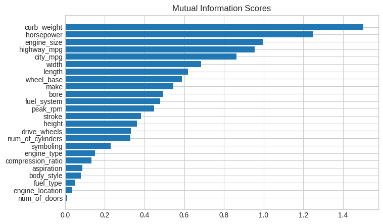

Data visualization is a great follow-up to a utility ranking. Let's take a closer look at a couple of these.

数据可视化是展示排名的一个很好的后续。 让我们仔细看看其中的几个。

As we might expect, the high-scoring curb_weight feature exhibits a strong relationship with price, the target.

正如我们所预料的，高分curb_weight特征与目标price表现出很强的关系。

# sns.relplot(x="curb_weight", y="price", data=df)
sns.regplot(x="curb_weight", y="price", data=df)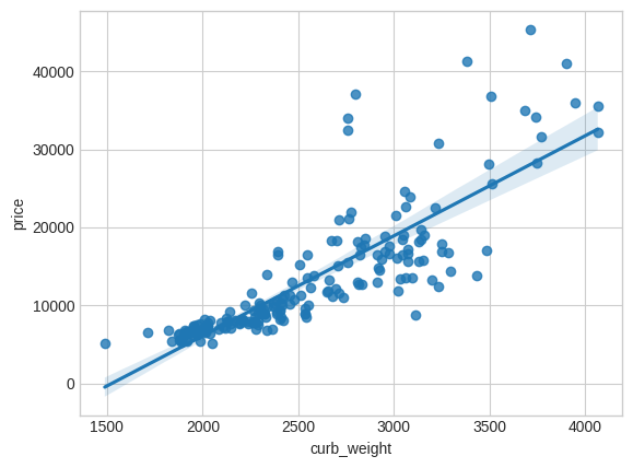

The fuel_type feature has a fairly low MI score, but as we can see from the figure, it clearly separates two price populations with different trends within the horsepower feature. This indicates that fuel_type contributes an interaction effect and might not be unimportant after all. Before deciding a feature is unimportant from its MI score, it's good to investigate any possible interaction effects -- domain knowledge can offer a lot of guidance here.

fuel_type特征的 MI 得分相当低，但从图中可以看出，它在horsepower特征中清楚地区分了具有不同趋势的两个price群体。 这表明fuel_type具有交互作用，并且可能很重要。 在根据 MI 分数确定某个功能是否重要之前，最好调查一下任何可能的交互影响 —— 该领域的知识可以在这里提供很多指导。

sns.lmplot(x="horsepower", y="price", hue="fuel_type", data=df);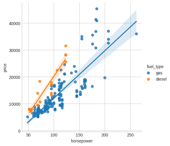

Data visualization is a great addition to your feature-engineering toolbox. Along with utility metrics like mutual information, visualizations like these can help you discover important relationships in your data. Check out our Data Visualization course to learn more!

数据可视化是对特征工程工具箱的一个很好的补充。 除了互信息等实用指标之外，此类可视化可以帮助您发现数据中的重要关系。 查看我们的数据可视化 课程以了解更多信息！

Your Turn

到你了

Rank the features of the Ames Housing dataset and choose your first set of features to start developing.

对 Ames Housing 数据集的 特征进行排序 ，并选择您的第一组特征来开始开发。