This notebook is an exercise in the Feature Engineering course. You can reference the tutorial at this link.

---

Introduction

介绍

In this exercise you'll identify an initial set of features in the Ames dataset to develop using mutual information scores and interaction plots.

在本练习中，您将确定 Ames 数据集中的一组初始特征，以使用互信息分数和交互图进行开发。

Run this cell to set everything up!

运行这个单元格来设置一切！

# Setup feedback system
from learntools.core import binder
binder.bind(globals())
from learntools.feature_engineering_new.ex2 import *

import matplotlib.pyplot as plt
import numpy as np
import pandas as pd
import seaborn as sns
from sklearn.feature_selection import mutual_info_regression

# Set Matplotlib defaults
plt.style.use("seaborn-v0_8-whitegrid")
plt.rc("figure", autolayout=True)
plt.rc(
    "axes",
    labelweight="bold",
    labelsize="large",
    titleweight="bold",
    titlesize=14,
    titlepad=10,
)

# Load data
df = pd.read_csv("../input/fe-course-data/ames.csv")

# Utility functions from Tutorial
def make_mi_scores(X, y):
    X = X.copy()
    for colname in X.select_dtypes(["object", "category"]):
        X[colname], _ = X[colname].factorize()
    # All discrete features should now have integer dtypes
    discrete_features = [pd.api.types.is_integer_dtype(t) for t in X.dtypes]
    mi_scores = mutual_info_regression(X, y, discrete_features=discrete_features, random_state=0)
    mi_scores = pd.Series(mi_scores, name="MI Scores", index=X.columns)
    mi_scores = mi_scores.sort_values(ascending=False)
    return mi_scores

def plot_mi_scores(scores):
    scores = scores.sort_values(ascending=True)
    width = np.arange(len(scores))
    ticks = list(scores.index)
    plt.barh(width, scores)
    plt.yticks(width, ticks)
    plt.title("Mutual Information Scores")

---

To start, let's review the meaning of mutual information by looking at a few features from the Ames dataset.

首先，让我们通过查看 Ames 数据集中的一些特征来回顾一下互信息的含义。

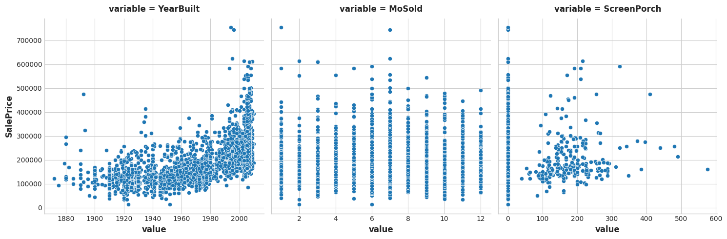
features = ["YearBuilt", "MoSold", "ScreenPorch"]
sns.relplot(
    x="value", y="SalePrice", col="variable", data=df.melt(id_vars="SalePrice", value_vars=features), facet_kws=dict(sharex=False),
);

1) Understand Mutual Information

1) 了解互信息

Based on the plots, which feature do you think would have the highest mutual information with SalePrice?

根据这些图，您认为哪个特征与SalePrice具有最高的互信息？

# View the solution (Run this cell to receive credit!)
q_1.check()

Correct:

Based on the plots, YearBuilt should have the highest MI score since knowing the year tends to constrain SalePrice to a smaller range of possible values. This is generally not the case for MoSold, however. Finally, since ScreenPorch is usually just one value, 0, on average it won't tell you much about SalePrice (though more than MoSold) .

---

The Ames dataset has seventy-eight features -- a lot to work with all at once! Fortunately, you can identify the features with the most potential.

Ames 数据集有 78 个特征——有很多特征需要同时处理！ 幸运的是，您可以识别出最有潜力的功能。

Use the make_mi_scores function (introduced in the tutorial) to compute mutual information scores for the Ames features:

使用 make_mi_scores 函数（在教程中介绍）计算 Ames 特征的互信息分数：

X = df.copy()
y = X.pop('SalePrice')

mi_scores = make_mi_scores(X, y)

Now examine the scores using the functions in this cell. Look especially at top and bottom ranks.

现在使用此单元格中的函数检查分数。 尤其要注意顶部和底部的排名。

print(mi_scores.head(20))
# print(mi_scores.tail(20))  # uncomment to see bottom 20

plt.figure(dpi=100, figsize=(8, 5))
plot_mi_scores(mi_scores.head(20))
# plot_mi_scores(mi_scores.tail(20))  # uncomment to see bottom 20

OverallQual     0.581262
Neighborhood    0.569813
GrLivArea       0.496909
YearBuilt       0.437939
GarageArea      0.415014
TotalBsmtSF     0.390280
GarageCars      0.381467
FirstFlrSF      0.368825
BsmtQual        0.364779
KitchenQual     0.326194
ExterQual       0.322390
YearRemodAdd    0.315402
MSSubClass      0.287131
GarageFinish    0.265440
FullBath        0.251693
Foundation      0.236115
LotFrontage     0.233334
GarageType      0.226117
FireplaceQu     0.221955
SecondFlrSF     0.200658
Name: MI Scores, dtype: float64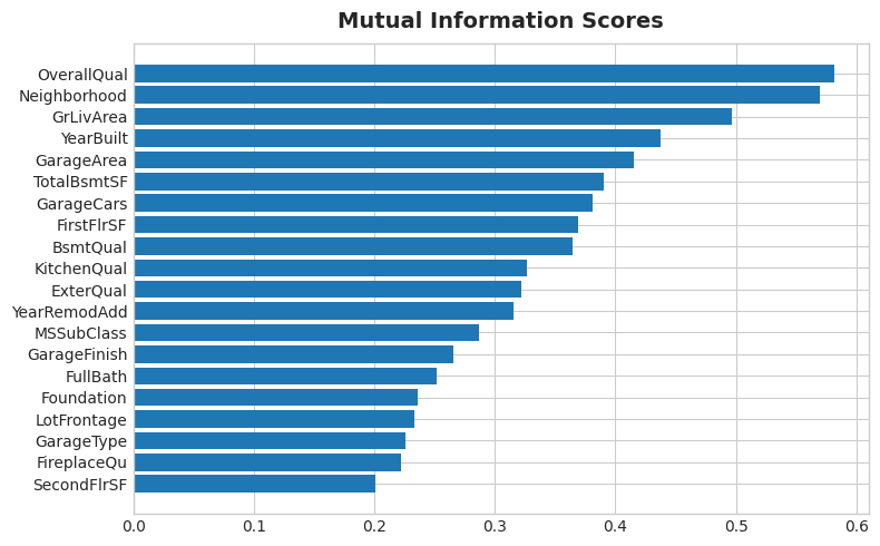

2) Examine MI Scores

2) 检查 MI 分数

Do the scores seem reasonable? Do the high scoring features represent things you'd think most people would value in a home? Do you notice any themes in what they describe?

分数看起来合理吗？ 高分功能是否代表了您认为大多数人会看重房屋的东西？ 您注意到他们所描述的主题吗？

# View the solution (Run this cell to receive credit!)
q_2.check()

Correct:

Some common themes among most of these features are:

• Location: Neighborhood
• Size: all of the Area and SF features, and counts like FullBath and GarageCars
• Quality: all of the Qual features
• Year: YearBuilt and YearRemodAdd
• Types: descriptions of features and styles like Foundation and GarageType

These are all the kinds of features you'll commonly see in real-estate listings (like on Zillow), It's good then that our mutual information metric scored them highly. On the other hand, the lowest ranked features seem to mostly represent things that are rare or exceptional in some way, and so wouldn't be relevant to the average home buyer.

---

In this step you'll investigate possible interaction effects for the BldgType feature. This feature describes the broad structure of the dwelling in five categories:

在此步骤中，您将研究BldgType功能可能的交互效果。 此功能将住宅的大致结构分为五类：

Bldg Type (Nominal): Type of dwelling
建筑类型（名义）：住宅类型

  1Fam    Single-family Detached  
  1Fam    单户独立屋
  2FmCon  Two-family Conversion; originally built as one-family dwelling
  2FmCon  二家转换； 最初是作为一家住宅建造的
  Duplx   Duplex
  Duplx   复式
  TwnhsE  Townhouse End Unit
  TwnhsE  联排别墅末端单元
  TwnhsI  Townhouse Inside Unit
  TwnhsI  联排别墅内部单位

The BldgType feature didn't get a very high MI score. A plot confirms that the categories in BldgType don't do a good job of distinguishing values in SalePrice (the distributions look fairly similar, in other words):

BldgType功能没有获得很高的 MI 分数。 一个图证实了BldgType中的类别不能很好地区分SalePrice中的值（换句话说，分布看起来非常相似）：

sns.catplot(x="BldgType", y="SalePrice", data=df, kind="boxen");

/opt/conda/lib/python3.10/site-packages/seaborn/categorical.py:1794: FutureWarning: use_inf_as_na option is deprecated and will be removed in a future version. Convert inf values to NaN before operating instead.
  with pd.option_context('mode.use_inf_as_na', True):
/opt/conda/lib/python3.10/site-packages/seaborn/categorical.py:1794: FutureWarning: use_inf_as_na option is deprecated and will be removed in a future version. Convert inf values to NaN before operating instead.
  with pd.option_context('mode.use_inf_as_na', True):
/opt/conda/lib/python3.10/site-packages/seaborn/categorical.py:1794: FutureWarning: use_inf_as_na option is deprecated and will be removed in a future version. Convert inf values to NaN before operating instead.
  with pd.option_context('mode.use_inf_as_na', True):
/opt/conda/lib/python3.10/site-packages/seaborn/categorical.py:1794: FutureWarning: use_inf_as_na option is deprecated and will be removed in a future version. Convert inf values to NaN before operating instead.
  with pd.option_context('mode.use_inf_as_na', True):
/opt/conda/lib/python3.10/site-packages/seaborn/categorical.py:1794: FutureWarning: use_inf_as_na option is deprecated and will be removed in a future version. Convert inf values to NaN before operating instead.
  with pd.option_context('mode.use_inf_as_na', True):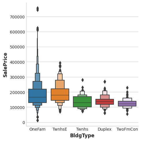

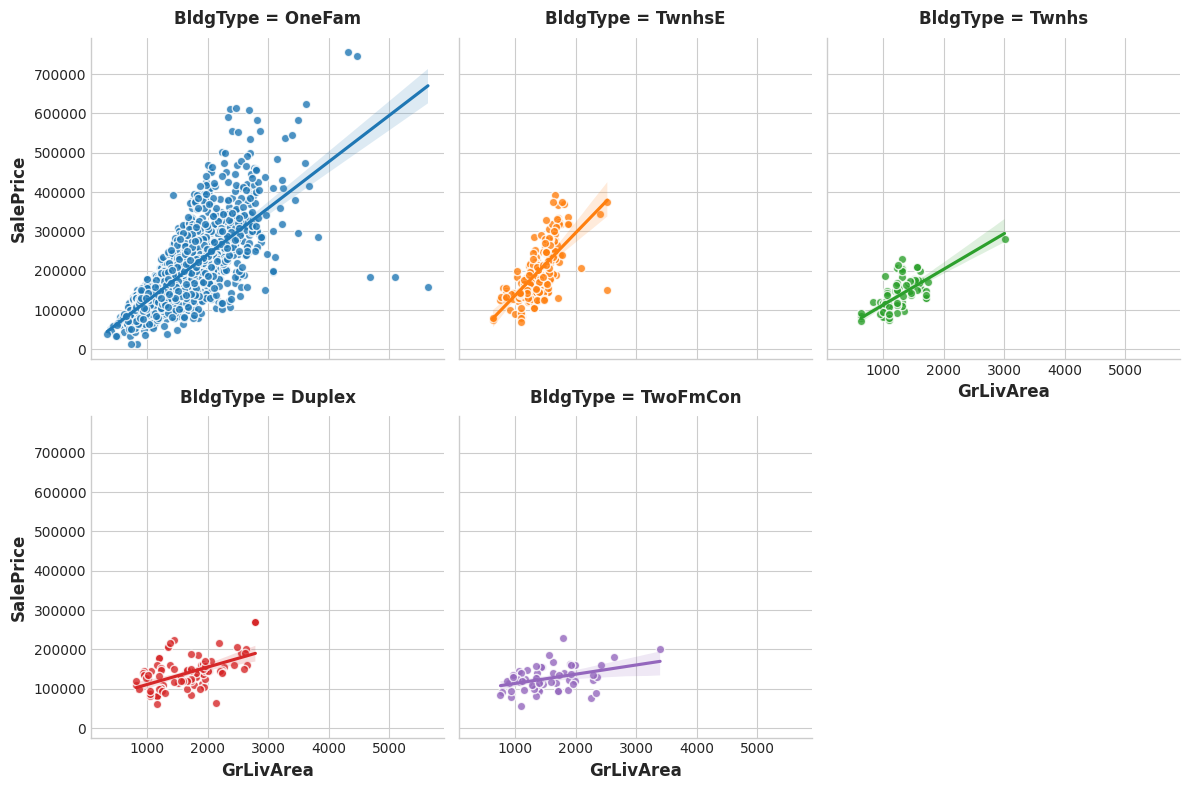
Still, the type of a dwelling seems like it should be important information. Investigate whether BldgType produces a significant interaction with either of the following:

尽管如此，住宅的类型似乎应该是重要的信息。 调查BldgType是否与以下任一项产生显着的交互：

GrLivArea   # Above ground living area
GrLivArea   # 地上生活区
MoSold      # Month sold
MoSold      # 已售出多少月

Run the following cell twice, the first time with feature = "GrLivArea" and the next time with feature="MoSold":

运行以下单元格两次，第一次使用 feature = "GrLivArea"，下一次使用 feature="MoSold"：

# YOUR CODE HERE: 
feature = "GrLivArea"

sns.lmplot(
    x=feature, y="SalePrice", hue="BldgType", col="BldgType",
    data=df, scatter_kws={"edgecolor": 'w'}, col_wrap=3, height=4,
);

# YOUR CODE HERE: 
feature = "MoSold"

sns.lmplot(
    x=feature, y="SalePrice", hue="BldgType", col="BldgType",
    data=df, scatter_kws={"edgecolor": 'w'}, col_wrap=3, height=4,
);

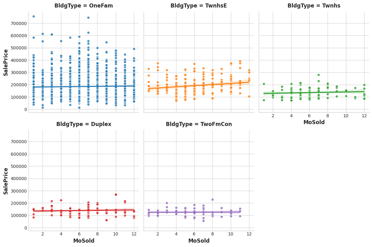
The trend lines being significantly different from one category to the next indicates an interaction effect.

一个类别与下一类别表明存在交互效应的趋势线存在明显的差距。

3) Discover Interactions

3) 发现互动

From the plots, does BldgType seem to exhibit an interaction effect with either GrLivArea or MoSold?

从图中来看，BldgType似乎与GrLivArea或MoSold表现出交互作用？

# View the solution (Run this cell to receive credit!)
q_3.check()

Correct:

The trends lines within each category of BldgType are clearly very different, indicating an interaction between these features. Since knowing BldgType tells us more about how GrLivArea relates to SalePrice, we should consider including BldgType in our feature set.

The trend lines for MoSold, however, are almost all the same. This feature hasn't become more informative for knowing BldgType.

A First Set of Development Features

第一组开发特征

Let's take a moment to make a list of features we might focus on. In the exercise in Lesson 3, you'll start to build up a more informative feature set through combinations of the original features you identified as having high potential.

让我们花点时间列出我们可能关注的特征。 在第 3 课的练习中，您将开始通过组合您认为具有高潜力的原始特征来构建信息更丰富的特征集。

You found that the ten features with the highest MI scores were:

您发现 MI 得分最高的 10 个特征是：

mi_scores.head(10)

OverallQual     0.581262
Neighborhood    0.569813
GrLivArea       0.496909
YearBuilt       0.437939
GarageArea      0.415014
TotalBsmtSF     0.390280
GarageCars      0.381467
FirstFlrSF      0.368825
BsmtQual        0.364779
KitchenQual     0.326194
Name: MI Scores, dtype: float64

Do you recognize the themes here? Location, size, and quality. You needn't restrict development to only these top features, but you do now have a good place to start. Combining these top features with other related features, especially those you've identified as creating interactions, is a good strategy for coming up with a highly informative set of features to train your model on.

你认出这里的主题了吗？ 位置、规模和质量。 您不必将开发仅限于这些顶级特征，但您现在确实有一个很好的起点。 将这些主要特征与其他相关特征（尤其是您确定用于创建交互的特征）相结合，是一个很好的策略，可以得出一组信息丰富的特征来训练您的模型。

Keep Going

继续前进

Start creating features and learn what kinds of transformations different models are most likely to benefit from.

开始创建特征并了解不同模型最有可能从哪些类型的转换中受益。