05.exercise-distributions【练习：分布图】

This notebook is an exercise in the Data Visualization course. You can reference the tutorial at this link.

---

In this exercise, you will use your new knowledge to propose a solution to a real-world scenario. To succeed, you will need to import data into Python, answer questions using the data, and generate histograms and density plots to understand patterns in the data.

在本练习中，您将使用新知识提出现实场景的解决方案。 为了成功，您需要将数据导入 Python，使用数据回答问题，并生成 直方图 和 密度图 以了解数据中的模式。

Scenario

场景

You'll work with a real-world dataset containing information collected from microscopic images of breast cancer tumors, similar to the image below.

您将使用一个真实世界的数据集，其中包含从乳腺癌肿瘤的显微图像收集的信息，类似于下图。

Each tumor has been labeled as either benign (noncancerous) or malignant (cancerous).

每个肿瘤都被标记为良性 (noncancerous) 或 恶性 (cancerous)。

To learn more about how this kind of data is used to create intelligent algorithms to classify tumors in medical settings, watch the short video at this link!

要详细了解如何使用此类数据创建智能算法来对医疗环境中的肿瘤进行分类，观看短视频在此链接 ！

Setup

设置

Run the next cell to import and configure the Python libraries that you need to complete the exercise.

运行下一个单元以导入和配置完成练习所需的 Python 库。

import pandas as pd
pd.plotting.register_matplotlib_converters()
import matplotlib.pyplot as plt
%matplotlib inline
import seaborn as sns
print("Setup Complete")

Setup Complete

The questions below will give you feedback on your work. Run the following cell to set up our feedback system.

以下问题将为您提供有关您工作的反馈。 运行以下单元格来设置我们的反馈系统。

# Set up code checking
import os
if not os.path.exists("../input/cancer_b.csv"):
    os.symlink("../input/data-for-datavis/cancer_b.csv", "../input/cancer_b.csv")
    os.symlink("../input/data-for-datavis/cancer_m.csv", "../input/cancer_m.csv")
from learntools.core import binder
binder.bind(globals())
from learntools.data_viz_to_coder.ex5 import *
print("Setup Complete")

Setup Complete

Step 1: Load the data

第 1 步：加载数据

In this step, you will load two data files.

在此步骤中，您将加载两个数据文件。

• Load the data file corresponding to benign tumors into a DataFrame called cancer_b_data. The corresponding filepath is cancer_b_filepath. Use the "Id" column to label the rows.
• 将与良性肿瘤相对应的数据文件加载到名为cancer_b_data的 DataFrame 中。 对应的文件路径是cancer_b_filepath。 使用Id列来标记行。
• Load the data file corresponding to malignant tumors into a DataFrame called cancer_m_data. The corresponding filepath is cancer_m_filepath. Use the "Id" column to label the rows.
• 将与 恶性 肿瘤相对应的数据文件加载到名为cancer_m_data的 DataFrame 中。 对应的文件路径是cancer_m_filepath。 使用Id列来标记行。

# Paths of the files to read
cancer_b_filepath = "../input/cancer_b.csv"
cancer_m_filepath = "../input/cancer_m.csv"

cancer_filepath = "../input/cancer.csv"

# Fill in the line below to read the (benign) file into a variable cancer_b_data
#cancer_b_data = ____

# Fill in the line below to read the (malignant) file into a variable cancer_m_data
#cancer_m_data = ____

cancer_b_data = pd.read_csv(cancer_b_filepath, index_col='Id')
cancer_m_data = pd.read_csv(cancer_m_filepath, index_col='Id')

cancer_data = pd.read_csv(cancer_filepath, index_col='Id')

# Run the line below with no changes to check that you've loaded the data correctly
step_1.check()

Correct

# Lines below will give you a hint or solution code
#step_1.hint()
step_1.solution()

Solution:

cancer_data = pd.read_csv(cancer_filepath, index_col="Id")

Step 2: Review the data

第 2 步：查看数据

Use a Python command to print the first 5 rows of the data for benign tumors.

使用 Python 命令打印良性肿瘤的前 5 行数据。

# Print the first five rows of the (benign) data
#____ # Your code here
cancer_b_data.head()

	Diagnosis	Radius (mean)	Texture (mean)	Perimeter (mean)	Area (mean)	Smoothness (mean)	Compactness (mean)	Concavity (mean)	Concave points (mean)	Symmetry (mean)	...	Radius (worst)	Texture (worst)	Perimeter (worst)	Area (worst)	Smoothness (worst)	Compactness (worst)	Concavity (worst)	Concave points (worst)	Symmetry (worst)	Fractal dimension (worst)
Id
8510426	B	13.540	14.36	87.46	566.3	0.09779	0.08129	0.06664	0.047810	0.1885	...	15.110	19.26	99.70	711.2	0.14400	0.17730	0.23900	0.12880	0.2977	0.07259
8510653	B	13.080	15.71	85.63	520.0	0.10750	0.12700	0.04568	0.031100	0.1967	...	14.500	20.49	96.09	630.5	0.13120	0.27760	0.18900	0.07283	0.3184	0.08183
8510824	B	9.504	12.44	60.34	273.9	0.10240	0.06492	0.02956	0.020760	0.1815	...	10.230	15.66	65.13	314.9	0.13240	0.11480	0.08867	0.06227	0.2450	0.07773
854941	B	13.030	18.42	82.61	523.8	0.08983	0.03766	0.02562	0.029230	0.1467	...	13.300	22.81	84.46	545.9	0.09701	0.04619	0.04833	0.05013	0.1987	0.06169
85713702	B	8.196	16.84	51.71	201.9	0.08600	0.05943	0.01588	0.005917	0.1769	...	8.964	21.96	57.26	242.2	0.12970	0.13570	0.06880	0.02564	0.3105	0.07409

5 rows × 31 columns

Use a Python command to print the first 5 rows of the data for malignant tumors.

使用Python命令打印恶性肿瘤的前5行数据。

# Print the first five rows of the (malignant) data
#____ # Your code here
cancer_m_data.head()

	Diagnosis	Radius (mean)	Texture (mean)	Perimeter (mean)	Area (mean)	Smoothness (mean)	Compactness (mean)	Concavity (mean)	Concave points (mean)	Symmetry (mean)	...	Radius (worst)	Texture (worst)	Perimeter (worst)	Area (worst)	Smoothness (worst)	Compactness (worst)	Concavity (worst)	Concave points (worst)	Symmetry (worst)	Fractal dimension (worst)
Id
842302	M	17.99	10.38	122.80	1001.0	0.11840	0.27760	0.3001	0.14710	0.2419	...	25.38	17.33	184.60	2019.0	0.1622	0.6656	0.7119	0.2654	0.4601	0.11890
842517	M	20.57	17.77	132.90	1326.0	0.08474	0.07864	0.0869	0.07017	0.1812	...	24.99	23.41	158.80	1956.0	0.1238	0.1866	0.2416	0.1860	0.2750	0.08902
84300903	M	19.69	21.25	130.00	1203.0	0.10960	0.15990	0.1974	0.12790	0.2069	...	23.57	25.53	152.50	1709.0	0.1444	0.4245	0.4504	0.2430	0.3613	0.08758
84348301	M	11.42	20.38	77.58	386.1	0.14250	0.28390	0.2414	0.10520	0.2597	...	14.91	26.50	98.87	567.7	0.2098	0.8663	0.6869	0.2575	0.6638	0.17300
84358402	M	20.29	14.34	135.10	1297.0	0.10030	0.13280	0.1980	0.10430	0.1809	...	22.54	16.67	152.20	1575.0	0.1374	0.2050	0.4000	0.1625	0.2364	0.07678

5 rows × 31 columns

In the datasets, each row corresponds to a different image. Each dataset has 31 different columns, corresponding to:

在数据集中，每一行对应于不同的图像。 每个数据集有 31 个不同的列，对应于：

• 1 column ('Diagnosis') that classifies tumors as either benign (which appears in the dataset as B) or malignant (M), and
• 1 列（'Diagnosis'）将肿瘤分类为良性（在数据集中显示为 B ）或恶性（ M ），以及
• 30 columns containing different measurements collected from the images.
• 30 列包含从图像中收集的不同测量值。

Use the first 5 rows of the data (for benign and malignant tumors) to answer the questions below.

使用前 5 行数据（良性和恶性肿瘤）回答以下问题。

# Fill in the line below: In the first five rows of the data for benign tumors, what is the
# largest value for 'Perimeter (mean)'?
#max_perim = ____
max_perim = cancer_b_data.head()['Perimeter (mean)'].max()

# Fill in the line below: What is the value for 'Radius (mean)' for the tumor with Id 842517?
#mean_radius = ____
# mean_radius = cancer_m_data.loc[842517]['Radius (mean)']
mean_radius = cancer_data.loc[8510824]['Radius (mean)']

# Check your answers
step_2.check()

Correct

# Lines below will give you a hint or solution code
# step_2.hint()
step_2.solution()

Solution:

# Print the first five rows of the data
cancer_data.head()
# In the first five rows of the data, what is the
# largest value for 'Perimeter (mean)'?
max_perim = 87.46
# What is the value for 'Radius (mean)' for the tumor with Id 8510824?
mean_radius = 9.504

Step 3: Investigating differences

步骤 3：调查差异

Part A

A 部分

Use the code cell below to create two histograms that show the distribution in values for 'Area (mean)' for both benign and malignant tumors. (To permit easy comparison, create a single figure containing both histograms in the code cell below.)

使用下面的代码单元创建两个直方图，显示良性肿瘤和恶性肿瘤的面积（平均值）值的分布。 （为了方便比较，请在下面的代码单元格中创建一个包含两个直方图的图形。）

pd.option_context('mode.use_inf_as_na', True)
# Histograms for benign and maligant tumors
#____ # Your code here (benign tumors)
#____ # Your code here (malignant tumors)

# sns.histplot(cancer_b_data['Area (mean)'], kde=False)
# sns.histplot(cancer_m_data['Area (mean)'], kde=False)

sns.histplot(data=cancer_data, x='Area (mean)', hue='Diagnosis')

# Check your answer
step_3.a.check()

/opt/conda/lib/python3.10/site-packages/seaborn/_oldcore.py:1119: FutureWarning: use_inf_as_na option is deprecated and will be removed in a future version. Convert inf values to NaN before operating instead.
  with pd.option_context('mode.use_inf_as_na', True):
/opt/conda/lib/python3.10/site-packages/seaborn/_oldcore.py:1075: FutureWarning: When grouping with a length-1 list-like, you will need to pass a length-1 tuple to get_group in a future version of pandas. Pass (name,) instead of name to silence this warning.
  data_subset = grouped_data.get_group(pd_key)
/opt/conda/lib/python3.10/site-packages/seaborn/_oldcore.py:1075: FutureWarning: When grouping with a length-1 list-like, you will need to pass a length-1 tuple to get_group in a future version of pandas. Pass (name,) instead of name to silence this warning.
  data_subset = grouped_data.get_group(pd_key)
/opt/conda/lib/python3.10/site-packages/seaborn/_oldcore.py:1075: FutureWarning: When grouping with a length-1 list-like, you will need to pass a length-1 tuple to get_group in a future version of pandas. Pass (name,) instead of name to silence this warning.
  data_subset = grouped_data.get_group(pd_key)

Correct

# Lines below will give you a hint or solution code
# step_3.a.hint()
step_3.a.solution_plot()

Solution:

# Histograms for benign and maligant tumors
sns.histplot(data=cancer_data, x='Area (mean)', hue='Diagnosis')

/opt/conda/lib/python3.10/site-packages/seaborn/_oldcore.py:1119: FutureWarning: use_inf_as_na option is deprecated and will be removed in a future version. Convert inf values to NaN before operating instead.
  with pd.option_context('mode.use_inf_as_na', True):
/opt/conda/lib/python3.10/site-packages/seaborn/_oldcore.py:1075: FutureWarning: When grouping with a length-1 list-like, you will need to pass a length-1 tuple to get_group in a future version of pandas. Pass (name,) instead of name to silence this warning.
  data_subset = grouped_data.get_group(pd_key)
/opt/conda/lib/python3.10/site-packages/seaborn/_oldcore.py:1075: FutureWarning: When grouping with a length-1 list-like, you will need to pass a length-1 tuple to get_group in a future version of pandas. Pass (name,) instead of name to silence this warning.
  data_subset = grouped_data.get_group(pd_key)
/opt/conda/lib/python3.10/site-packages/seaborn/_oldcore.py:1075: FutureWarning: When grouping with a length-1 list-like, you will need to pass a length-1 tuple to get_group in a future version of pandas. Pass (name,) instead of name to silence this warning.
  data_subset = grouped_data.get_group(pd_key)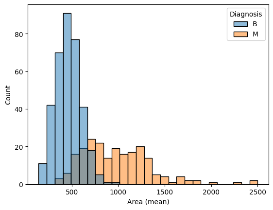

Part B

B 部分

A researcher approaches you for help with identifying how the 'Area (mean)' column can be used to understand the difference between benign and malignant tumors. Based on the histograms above,

研究人员向您寻求帮助，以确定如何使用'Area (mean)'列来了解良性肿瘤和恶性肿瘤之间的差异。 根据上面的直方图，

• Do malignant tumors have higher or lower values for 'Area (mean)' (relative to benign tumors), on average?
• 平均而言，恶性肿瘤的'Area (mean)'值（相对于良性肿瘤）是否较高或较低？
• Which tumor type seems to have a larger range of potential values?
• 哪种肿瘤类型似乎具有更大范围的潜在价值？

#step_3.b.hint()

# Check your answer (Run this code cell to receive credit!)
step_3.b.solution()

Solution: Malignant tumors have higher values for 'Area (mean)', on average. Malignant tumors have a larger range of potential values.

Step 4: A very useful column

步骤 4：非常有用的专栏

Part A

A 部分

Use the code cell below to create two KDE plots that show the distribution in values for 'Radius (worst)' for both benign and malignant tumors. (To permit easy comparison, create a single figure containing both KDE plots in the code cell below.)

使用下面的代码单元创建两个 KDE 图，显示良性肿瘤和恶性肿瘤的'Radius (worst)' 值的分布。 （为了方便比较，请在下面的代码单元格中创建一个包含两个 KDE 图的单个图形。）

# KDE plots for benign and malignant tumors
#____ # Your code here (benign tumors)
#____ # Your code here (malignant tumors)
# sns.kdeplot(cancer_b_data['Radius (worst)'], label='Benign')
# sns.kdeplot(cancer_m_data['Radius (worst)'], label='Malignant')
# plt.legend()

sns.kdeplot(data=cancer_data, x='Radius (worst)', hue='Diagnosis', fill=True)

# Check your answer
step_4.a.check()

/opt/conda/lib/python3.10/site-packages/seaborn/_oldcore.py:1119: FutureWarning: use_inf_as_na option is deprecated and will be removed in a future version. Convert inf values to NaN before operating instead.
  with pd.option_context('mode.use_inf_as_na', True):
/opt/conda/lib/python3.10/site-packages/seaborn/_oldcore.py:1075: FutureWarning: When grouping with a length-1 list-like, you will need to pass a length-1 tuple to get_group in a future version of pandas. Pass (name,) instead of name to silence this warning.
  data_subset = grouped_data.get_group(pd_key)
/opt/conda/lib/python3.10/site-packages/seaborn/_oldcore.py:1075: FutureWarning: When grouping with a length-1 list-like, you will need to pass a length-1 tuple to get_group in a future version of pandas. Pass (name,) instead of name to silence this warning.
  data_subset = grouped_data.get_group(pd_key)
/opt/conda/lib/python3.10/site-packages/seaborn/_oldcore.py:1075: FutureWarning: When grouping with a length-1 list-like, you will need to pass a length-1 tuple to get_group in a future version of pandas. Pass (name,) instead of name to silence this warning.
  data_subset = grouped_data.get_group(pd_key)

Correct

# Lines below will give you a hint or solution code
#step_4.a.hint()
step_4.a.solution_plot()

Solution:

# KDE plots for benign and malignant tumors
sns.kdeplot(data=cancer_data, x='Radius (worst)', hue='Diagnosis', shade=True)

/opt/conda/lib/python3.10/site-packages/learntools/data_viz_to_coder/ex5.py:83: FutureWarning: 

shade is now deprecated in favor of fill; setting fill=True.
This will become an error in seaborn v0.14.0; please update your code.

  sns.kdeplot(data=df, x='Radius (worst)', hue='Diagnosis', shade=True)
/opt/conda/lib/python3.10/site-packages/seaborn/_oldcore.py:1119: FutureWarning: use_inf_as_na option is deprecated and will be removed in a future version. Convert inf values to NaN before operating instead.
  with pd.option_context('mode.use_inf_as_na', True):
/opt/conda/lib/python3.10/site-packages/seaborn/_oldcore.py:1075: FutureWarning: When grouping with a length-1 list-like, you will need to pass a length-1 tuple to get_group in a future version of pandas. Pass (name,) instead of name to silence this warning.
  data_subset = grouped_data.get_group(pd_key)
/opt/conda/lib/python3.10/site-packages/seaborn/_oldcore.py:1075: FutureWarning: When grouping with a length-1 list-like, you will need to pass a length-1 tuple to get_group in a future version of pandas. Pass (name,) instead of name to silence this warning.
  data_subset = grouped_data.get_group(pd_key)
/opt/conda/lib/python3.10/site-packages/seaborn/_oldcore.py:1075: FutureWarning: When grouping with a length-1 list-like, you will need to pass a length-1 tuple to get_group in a future version of pandas. Pass (name,) instead of name to silence this warning.
  data_subset = grouped_data.get_group(pd_key)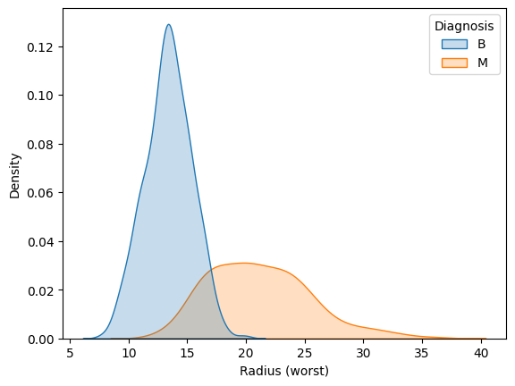

Part B

B 部分

A hospital has recently started using an algorithm that can diagnose tumors with high accuracy. Given a tumor with a value for 'Radius (worst)' of 25, do you think the algorithm is more likely to classify the tumor as benign or malignant?

一家医院最近开始使用一种可以高精度诊断肿瘤的算法。 给定'Radius (worst)' 值为 25 的肿瘤，您认为算法更有可能将肿瘤分类为良性还是恶性？

#step_4.b.hint()

# Check your answer (Run this code cell to receive credit!)
step_4.b.solution()

Solution: The algorithm is more likely to classify the tumor as malignant. This is because the curve for malignant tumors is much higher than the curve for benign tumors around a value of 25 -- and an algorithm that gets high accuracy is likely to make decisions based on this pattern in the data.

该算法更有可能将肿瘤分类为恶性。 这是因为恶性肿瘤的曲线比良性肿瘤的曲线高得多，约为 25，并且获得高精度的算法可能会根据数据中的这种模式做出决策。

Keep going

继续前进

Review all that you've learned and explore how to further customize your plots in the next tutorial!

回顾您所学到的所有知识，并在下一个教程中探索如何进一步自定义绘图 ！