This notebook is an exercise in the Feature Engineering course. You can reference the tutorial at this link.

---

Introduction

介绍

In this exercise, you'll work through several applications of PCA to the Ames dataset.

在本练习中，您将在 Ames 数据集上完成 PCA 的多种应用。

Run this cell to set everything up!

运行这个单元格来设置一切！

# Setup feedback system
from learntools.core import binder
binder.bind(globals())
from learntools.feature_engineering_new.ex5 import *

import matplotlib.pyplot as plt
import numpy as np
import pandas as pd
import seaborn as sns
from sklearn.decomposition import PCA
from sklearn.feature_selection import mutual_info_regression
from sklearn.model_selection import cross_val_score
from xgboost import XGBRegressor

# Set Matplotlib defaults
plt.style.use("seaborn-v0_8-whitegrid")
plt.rc("figure", autolayout=True)
plt.rc(
    "axes",
    labelweight="bold",
    labelsize="large",
    titleweight="bold",
    titlesize=14,
    titlepad=10,
)

def apply_pca(X, standardize=True):
    # Standardize
    if standardize:
        X = (X - X.mean(axis=0)) / X.std(axis=0)
    # Create principal components
    pca = PCA()
    X_pca = pca.fit_transform(X)
    # Convert to dataframe
    component_names = [f"PC{i+1}" for i in range(X_pca.shape[1])]
    X_pca = pd.DataFrame(X_pca, columns=component_names)
    # Create loadings
    loadings = pd.DataFrame(
        pca.components_.T,  # transpose the matrix of loadings
        columns=component_names,  # so the columns are the principal components
        index=X.columns,  # and the rows are the original features
    )
    return pca, X_pca, loadings

def plot_variance(pca, width=8, dpi=100):
    # Create figure
    fig, axs = plt.subplots(1, 2)
    n = pca.n_components_
    grid = np.arange(1, n + 1)
    # Explained variance
    evr = pca.explained_variance_ratio_
    axs[0].bar(grid, evr)
    axs[0].set(
        xlabel="Component", title="% Explained Variance", ylim=(0.0, 1.0)
    )
    # Cumulative Variance
    cv = np.cumsum(evr)
    axs[1].plot(np.r_[0, grid], np.r_[0, cv], "o-")
    axs[1].set(
        xlabel="Component", title="% Cumulative Variance", ylim=(0.0, 1.0)
    )
    # Set up figure
    fig.set(figwidth=8, dpi=100)
    return axs

def make_mi_scores(X, y):
    X = X.copy()
    for colname in X.select_dtypes(["object", "category"]):
        X[colname], _ = X[colname].factorize()
    # All discrete features should now have integer dtypes
    discrete_features = [pd.api.types.is_integer_dtype(t) for t in X.dtypes]
    mi_scores = mutual_info_regression(X, y, discrete_features=discrete_features, random_state=0)
    mi_scores = pd.Series(mi_scores, name="MI Scores", index=X.columns)
    mi_scores = mi_scores.sort_values(ascending=False)
    return mi_scores

def score_dataset(X, y, model=XGBRegressor()):
    # Label encoding for categoricals
    for colname in X.select_dtypes(["category", "object"]):
        X[colname], _ = X[colname].factorize()
    # Metric for Housing competition is RMSLE (Root Mean Squared Log Error)
    score = cross_val_score(
        model, X, y, cv=5, scoring="neg_mean_squared_log_error",
    )
    score = -1 * score.mean()
    score = np.sqrt(score)
    return score

df = pd.read_csv("../input/fe-course-data/ames.csv")

Let's choose a few features that are highly correlated with our target, SalePrice.

让我们选择一些与我们的目标SalePrice高度相关的特征。

features = [
    "GarageArea",
    "YearRemodAdd",
    "TotalBsmtSF",
    "GrLivArea",
]

print("Correlation with SalePrice:\n")
print(df[features].corrwith(df.SalePrice))

Correlation with SalePrice:

GarageArea      0.640138
YearRemodAdd    0.532974
TotalBsmtSF     0.632529
GrLivArea       0.706780
dtype: float64

We'll rely on PCA to untangle the correlational structure of these features and suggest relationships that might be usefully modeled with new features.

我们将依靠 PCA 来理清这些特征的相关结构，并提出可以用于建模的新特征。

Run this cell to apply PCA and extract the loadings.

运行此单元以应用 PCA 并提取负载。

X = df.copy()
y = X.pop("SalePrice")
X = X.loc[:, features]

# `apply_pca`, defined above, reproduces the code from the tutorial
pca, X_pca, loadings = apply_pca(X)
print(loadings)

                   PC1       PC2       PC3       PC4
GarageArea    0.541229  0.102375 -0.038470  0.833733
YearRemodAdd  0.427077 -0.886612 -0.049062 -0.170639
TotalBsmtSF   0.510076  0.360778 -0.666836 -0.406192
GrLivArea     0.514294  0.270700  0.742592 -0.332837

1) Interpret Component Loadings

1) 解释成分负载

Look at the loadings for components PC1 and PC3. Can you think of a description of what kind of contrast each component has captured? After you've thought about it, run the next cell for a solution.

查看成分PC1和PC3的负载。 您能描述一下每个组件所捕捉到的对比类型吗？ 想完之后，运行下一个单元格来寻找解决方案。

# View the solution (Run this cell to receive credit!)
q_1.check()

Correct:

The first component, PC1, seems to be a kind of "size" component, similar to what we saw in the tutorial: all of the features have the same sign (positive), indicating that this component is describing a contrast between houses having large values and houses having small values for these features.

The interpretation of the third component PC3 is a little trickier. The features GarageArea and YearRemodAdd both have near-zero loadings, so let's ignore those. This component is mostly about TotalBsmtSF and GrLivArea. It describes a contrast between houses with a lot of living area but small (or non-existant) basements, and the opposite: small houses with large basements.

第一个分量 PC1 似乎是一种大小分量，类似于我们在教程中看到的：所有特征都具有相同的符号（正），表明该分量描述的是具有较大尺寸的房屋之间的对比 值和这些特征的值较小的房屋。

第三个分量 PC3 的解释有点棘手。 GarageArea 和 YearRemodAdd 功能的负载都接近于零，所以让我们忽略它们。 该组件主要是关于 TotalBsmtSF 和 GrLivArea。 它描述了具有大量起居区但地下室较小（或不存在）的房屋与相反的房屋：具有大地下室的小房屋之间的对比。

---

Your goal in this question is to use the results of PCA to discover one or more new features that improve the performance of your model. One option is to create features inspired by the loadings, like we did in the tutorial. Another option is to use the components themselves as features (that is, add one or more columns of X_pca to X).

您在此问题中的目标是使用 PCA 结果发现一个或多个可提高模型性能的新特征。 一种选择是创建受载荷启发的特征，就像我们在教程中所做的那样。 另一种选择是使用组件本身作为特征（即，将X_pca的一列或多列添加到X）。

2) Create New Features

2) 创建新特征

Add one or more new features to the dataset X. For a correct solution, get a validation score below 0.140 RMSLE. (If you get stuck, feel free to use the hint below!)

向数据集X添加一项或多项新功能。 要获得正确的解决方案，请获得低于 0.140 RMSLE 的验证分数。 （如果您遇到困难，请随时使用下面的提示！）

X = df.copy()
y = X.pop("SalePrice")

# YOUR CODE HERE: Add new features to X.
# ____
# X = X.join(X_pca)
X["Feature5"] = X.GrLivArea + X.TotalBsmtSF
X["Feature2"] = X.YearRemodAdd * X.TotalBsmtSF * .9

score = score_dataset(X, y)
print(f"Your score: {score:.5f} RMSLE")

# Check your answer
q_2.check()

Your score: 0.13792 RMSLE

Correct:

Here are two possible solutions, though you might have been able to find others.

# Solution 1: Inspired by loadings
X = df.copy()
y = X.pop("SalePrice")

X["Feature1"] = X.GrLivArea + X.TotalBsmtSF
X["Feature2"] = X.YearRemodAdd * X.TotalBsmtSF

score = score_dataset(X, y)
print(f"Your score: {score:.5f} RMSLE")

# Solution 2: Uses components
X = df.copy()
y = X.pop("SalePrice")

X = X.join(X_pca)
score = score_dataset(X, y)
print(f"Your score: {score:.5f} RMSLE")

# Lines below will give you a hint or solution code
q_2.hint()
q_2.solution()

Hint: Try using the make_mi_scores function on X_pca to find out which components might have the most potential. Then look at the loadings to see what kinds of relationships among the features might be important.

Alternatively, you could use the components themselves. Try joining the highest scoring components from X_pca to X, or just join all of X_pca to X.

Solution: Here are two possible solutions, though you might have been able to find others.

# Solution 1: Inspired by loadings
X = df.copy()
y = X.pop("SalePrice")

X["Feature1"] = X.GrLivArea + X.TotalBsmtSF
X["Feature2"] = X.YearRemodAdd * X.TotalBsmtSF

score = score_dataset(X, y)
print(f"Your score: {score:.5f} RMSLE")

# Solution 2: Uses components
X = df.copy()
y = X.pop("SalePrice")

X = X.join(X_pca)
score = score_dataset(X, y)
print(f"Your score: {score:.5f} RMSLE")

---

The next question explores a way you can use PCA to detect outliers in the dataset (meaning, data points that are unusually extreme in some way). Outliers can have a detrimental effect on model performance, so it's good to be aware of them in case you need to take corrective action. PCA in particular can show you anomalous variation which might not be apparent from the original features: neither small houses nor houses with large basements are unusual, but it is unusual for small houses to have large basements. That's the kind of thing a principal component can show you.

下一个问题探讨了一种使用 PCA 检测数据集中的异常值（即在某种程度上异常极端的数据点）的方法。 异常值可能会对模型性能产生不利影响，因此最好了解它们，以防您需要采取纠正措施。 PCA 尤其可以向您显示异常的变化，这种变化在原始特征中可能并不明显：小房子和带有大地下室的房子都不是不寻常的，但小房子有大地下室是不寻常的。 这就是主成分可以向您展示的东西。

Run the next cell to show distribution plots for each of the principal components you created above.

运行下一个单元格以显示您在上面创建的每个主成分的分布图。

sns.catplot(
    y="value",
    col="variable",
    data=X_pca.melt(),
    kind='boxen',
    sharey=False,
    col_wrap=2,
);

/opt/conda/lib/python3.10/site-packages/seaborn/categorical.py:1794: FutureWarning: use_inf_as_na option is deprecated and will be removed in a future version. Convert inf values to NaN before operating instead.
  with pd.option_context('mode.use_inf_as_na', True):
/opt/conda/lib/python3.10/site-packages/seaborn/categorical.py:1794: FutureWarning: use_inf_as_na option is deprecated and will be removed in a future version. Convert inf values to NaN before operating instead.
  with pd.option_context('mode.use_inf_as_na', True):
/opt/conda/lib/python3.10/site-packages/seaborn/categorical.py:1794: FutureWarning: use_inf_as_na option is deprecated and will be removed in a future version. Convert inf values to NaN before operating instead.
  with pd.option_context('mode.use_inf_as_na', True):
/opt/conda/lib/python3.10/site-packages/seaborn/categorical.py:1794: FutureWarning: use_inf_as_na option is deprecated and will be removed in a future version. Convert inf values to NaN before operating instead.
  with pd.option_context('mode.use_inf_as_na', True):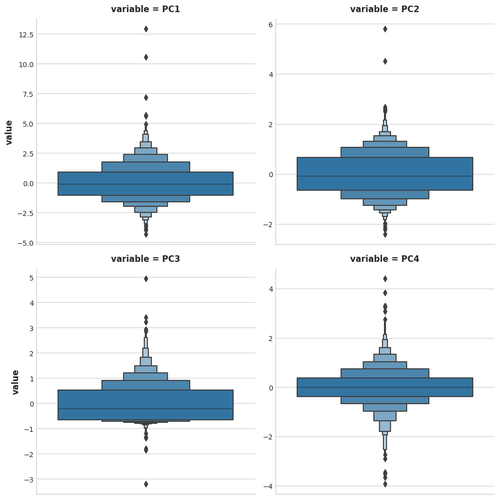

As you can see, in each of the components there are several points lying at the extreme ends of the distributions -- outliers, that is.

正如您所看到的，在每个成分中，都有几个点位于分布的最末端——即异常值。

Now run the next cell to see those houses that sit at the extremes of a component:

现在运行下一个单元格来查看位于组件极端的那些房屋：

# You can change PC1 to PC2, PC3, or PC4
component = "PC1"

idx = X_pca[component].sort_values(ascending=False).index
df.loc[idx, ["SalePrice", "Neighborhood", "SaleCondition"] + features]

	SalePrice	Neighborhood	SaleCondition	GarageArea	YearRemodAdd	TotalBsmtSF	GrLivArea
1498	160000	Edwards	Partial	1418.0	2008	6110.0	5642.0
2180	183850	Edwards	Partial	1154.0	2009	5095.0	5095.0
2181	184750	Edwards	Partial	884.0	2008	3138.0	4676.0
1760	745000	Northridge	Abnorml	813.0	1996	2396.0	4476.0
1767	755000	Northridge	Normal	832.0	1995	2444.0	4316.0
...	...	...	...	...	...	...	...
662	59000	Old_Town	Normal	0.0	1950	416.0	599.0
2679	80500	Brookside	Normal	0.0	1950	0.0	912.0
2879	51689	Iowa_DOT_and_Rail_Road	Abnorml	0.0	1950	0.0	729.0
780	63900	Sawyer	Normal	0.0	1950	0.0	660.0
1901	39300	Brookside	Normal	0.0	1950	0.0	334.0

2930 rows × 7 columns

3) Outlier Detection

3) 异常值检测

Do you notice any patterns in the extreme values? Does it seem like the outliers are coming from some special subset of the data?

您是否注意到极值中有任何模式？ 离群值似乎来自数据的某些特殊子集吗？

After you've thought about your answer, run the next cell for the solution and some discussion.

考虑完答案后，运行下一个单元格以获取解决方案并进行一些讨论。

# View the solution (Run this cell to receive credit!)
q_3.check()

Correct:

Notice that there are several dwellings listed as Partial sales in the Edwards neighborhood that stand out. A partial sale is what occurs when there are multiple owners of a property and one or more of them sell their "partial" ownership of the property.

These kinds of sales are often happen during the settlement of a family estate or the dissolution of a business and aren't advertised publicly. If you were trying to predict the value of a house on the open market, you would probably be justified in removing sales like these from your dataset -- they are truly outliers.

请注意，爱德华兹社区中有几处被列为部分销售的住宅非常引人注目。 部分出售是指一处房产有多个所有者，并且其中一个或多个所有者出售其对该房产的部分所有权时发生的情况。

此类出售通常发生在家庭财产清算或企业解散期间，并且不会公开宣传。 如果您试图预测公开市场上房屋的价值，您可能有理由从数据集中删除此类销售 - 它们确实是异常值。

Keep Going

继续前进

Apply target encoding to give a boost to categorical features.

应用目标编码 来增强分类特征。