This notebook is an exercise in the Feature Engineering course. You can reference the tutorial at this link.
Introduction
介绍
In this exercise, you'll apply target encoding to features in the Ames dataset.
在本练习中,您将对 Ames 数据集中的特征应用目标编码。
Run this cell to set everything up!
运行这个单元格来设置一切!
# Setup feedback system
from learntools.core import binder
binder.bind(globals())
from learntools.feature_engineering_new.ex6 import *

import matplotlib.pyplot as plt
import numpy as np
import pandas as pd
import seaborn as sns
import warnings
from category_encoders import MEstimateEncoder
from sklearn.model_selection import cross_val_score
from xgboost import XGBRegressor

# Set Matplotlib defaults
plt.style.use("seaborn-v0_8-whitegrid")
plt.rc("figure", autolayout=True)
plt.rc(
    "axes",
    labelweight="bold",
    labelsize="large",
    titleweight="bold",
    titlesize=14,
    titlepad=10,
)
warnings.filterwarnings('ignore')

def score_dataset(X, y, model=XGBRegressor()):
    # Label encoding for categoricals
    for colname in X.select_dtypes(["category", "object"]):
        X[colname], _ = X[colname].factorize()
    # Metric for Housing competition is RMSLE (Root Mean Squared Log Error)
    score = cross_val_score(
        model, X, y, cv=5, scoring="neg_mean_squared_log_error",
    )
    score = -1 * score.mean()
    score = np.sqrt(score)
    return score

df = pd.read_csv("../input/fe-course-data/ames.csv")
First you'll need to choose which features you want to apply a target encoding to. Categorical features with a large number of categories are often good candidates. Run this cell to see how many categories each categorical feature in the Ames dataset has.
首先,您需要选择要应用目标编码的特征。 具有大量类别的分类特征通常是很好的候选者。 运行此单元格以查看 Ames 数据集中每个分类特征有多少个类别。
df.select_dtypes(["object"]).nunique()MSSubClass 16
MSZoning 7
Street 2
Alley 3
LotShape 4
LandContour 4
Utilities 3
LotConfig 5
LandSlope 3
Neighborhood 28
Condition1 9
Condition2 8
BldgType 5
HouseStyle 8
OverallQual 10
OverallCond 9
RoofStyle 6
RoofMatl 8
Exterior1st 16
Exterior2nd 17
MasVnrType 4
ExterQual 4
ExterCond 5
Foundation 6
BsmtQual 6
BsmtCond 6
BsmtExposure 5
BsmtFinType1 7
BsmtFinType2 7
Heating 6
HeatingQC 5
CentralAir 2
Electrical 6
KitchenQual 5
Functional 8
FireplaceQu 6
GarageType 7
GarageFinish 4
GarageQual 6
GarageCond 6
PavedDrive 3
PoolQC 5
Fence 5
MiscFeature 5
SaleType 10
SaleCondition 6
dtype: int64We talked about how the M-estimate encoding uses smoothing to improve estimates for rare categories. To see how many times a category occurs in the dataset, you can use the value_counts method. This cell shows the counts for SaleType, but you might want to consider others as well.
我们讨论了 M 估计编码如何使用平滑来改进对稀有类别的估计。 要查看某个类别在数据集中出现的次数,可以使用value_counts方法。 此单元格显示SaleType的计数,但您可能还需要考虑其他单元格。
df["SaleType"].value_counts()SaleType
WD 2536
New 239
COD 87
ConLD 26
CWD 12
ConLI 9
ConLw 8
Oth 7
Con 5
VWD 1
Name: count, dtype: int641) Choose Features for Encoding
1) 选择编码特征
Which features did you identify for target encoding? After you've thought about your answer, run the next cell for some discussion.
您确定了目标编码的哪些特征? 考虑完答案后,运行下一个单元格进行一些讨论。
# View the solution (Run this cell to receive credit!)
q_1.check()
Correct:
The Neighborhood feature looks promising. It has the most categories of any feature, and several categories are rare. Others that could be worth considering are SaleType, MSSubClass, Exterior1st, Exterior2nd. In fact, almost any of the nominal features would be worth trying because of the prevalence of rare categories.
Neighborhood特征看起来很有前途。 它的类别是所有特征中最多的,并且有几个类别是罕见的。 其他可能值得考虑的有 SaleType、MSSubClass、Exterior1st、Exterior2nd。 事实上,由于稀有类别的普遍存在,几乎所有名义特征都值得尝试。
Now you'll apply a target encoding to your choice of feature. As we discussed in the tutorial, to avoid overfitting, we need to fit the encoder on data heldout from the training set. Run this cell to create the encoding and training splits:
现在,您将应用目标编码到您选择的特征。 正如我们在教程中讨论的,为了避免过拟合,我们需要在训练集中分割出的数据上进行编码器拟合。 运行此单元以创建编码和分割训练集:
# Encoding split
X_encode = df.sample(frac=0.20, random_state=0)
y_encode = X_encode.pop("SalePrice")

# Training split
X_pretrain = df.drop(X_encode.index)
y_train = X_pretrain.pop("SalePrice")
2) Apply M-Estimate Encoding
2) 应用 M-估计编码
Apply a target encoding to your choice of categorical features. Also choose a value for the smoothing parameter m (any value is okay for a correct answer).
将目标编码应用于您选择的分类特征。 还要为平滑参数m选择一个值(任何值都可以得到正确答案)。
# YOUR CODE HERE: Create the MEstimateEncoder
# Choose a set of features to encode and a value for m
# encoder = ____
encoder = MEstimateEncoder(
    cols=["Neighborhood"],
    m=1.0,
)

# Fit the encoder on the encoding split
# ____
encoder.fit(X_encode, y_encode)

# Encode the training split
X_train = encoder.transform(X_pretrain, y_train)

# Check your answer
q_2.check()
Correct
# Lines below will give you a hint or solution code
#q_2.hint()
q_2.solution()
Solution:
encoder = MEstimateEncoder(
    cols=["Neighborhood"],
    m=1.0,
)

# Fit the encoder on the encoding split
encoder.fit(X_encode, y_encode)

# Encode the training split
X_train = encoder.transform(X_pretrain, y_train)
If you'd like to see how the encoded feature compares to the target, you can run this cell:
如果您想查看编码特征与目标的比较情况,可以运行此单元格:
feature = encoder.cols

plt.figure(dpi=90)
ax = sns.distplot(y_train, kde=True, hist=False)
ax = sns.distplot(X_train[feature], color='r', ax=ax, hist=True, kde=False, norm_hist=True)
ax.set_xlabel("SalePrice");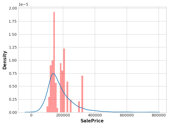
From the distribution plots, does it seem like the encoding is informative?
从分布图来看,编码是否提供了丰富的信息?
And this cell will show you the score of the encoded set compared to the original set:
此单元格将显示编码集与原始集相比的分数:
X = df.copy()
y = X.pop("SalePrice")
score_base = score_dataset(X, y)
score_new = score_dataset(X_train, y_train)

print(f"Baseline Score: {score_base:.4f} RMSLE")
print(f"Score with Encoding: {score_new:.4f} RMSLE")
Baseline Score: 0.1434 RMSLE
Score with Encoding: 0.1434 RMSLEDo you think that target encoding was worthwhile in this case? Depending on which feature or features you chose, you may have ended up with a score significantly worse than the baseline. In that case, it's likely the extra information gained by the encoding couldn't make up for the loss of data used for the encoding.
您认为在这种情况下目标编码值得吗? 根据您选择的特征,您最终的分数可能明显低于基线。 在这种情况下,通过编码获得的额外信息可能无法弥补用于编码的数据损失。
In this question, you'll explore the problem of overfitting with target encodings. This will illustrate this importance of training fitting target encoders on data held-out from the training set.
在这个问题中,您将探讨目标编码的过度拟合问题。 这将说明在训练集中分割的数据上训练拟合目标编码器的重要性。
So let's see what happens when we fit the encoder and the model on the same dataset. To emphasize how dramatic the overfitting can be, we'll mean-encode a feature that should have no relationship with SalePrice, a count: 0, 1, 2, 3, 4, 5, ....
因此,让我们看看当我们将编码器和模型拟合到相同数据集上时会发生什么。 为了强调过度拟合的严重性,我们将编码一个与SalePrice没有关系的特征,计数:0, 1, 2, 3, 4, 5, ...。
# Try experimenting with the smoothing parameter m
# Try 0, 1, 5, 50
m = 0

X = df.copy()
y = X.pop('SalePrice')

# Create an uninformative feature
X["Count"] = range(len(X))
# 实际上需要一个重复值来规避 MEstimateEncoder 中的错误检查
X["Count"][1] = 0  # actually need one duplicate value to circumvent error-checking in MEstimateEncoder

# fit and transform on the same dataset
encoder = MEstimateEncoder(cols="Count", m=m)
X = encoder.fit_transform(X, y)

# Results
score =  score_dataset(X, y)
print(f"Score: {score:.4f} RMSLE")
Score: 0.0375 RMSLEAlmost a perfect score!
几乎是完美!
plt.figure(dpi=90)
ax = sns.distplot(y, kde=True, hist=False)
ax = sns.distplot(X["Count"], color='r', ax=ax, hist=True, kde=False, norm_hist=True)
ax.set_xlabel("SalePrice");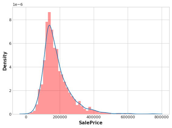
And the distributions are almost exactly the same, too.
而且分布也几乎完全相同。
3) Overfitting with Target Encoders
3) 目标编码器过度拟合
Based on your understanding of how mean-encoding works, can you explain how XGBoost was able to get an almost a perfect fit after mean-encoding the count feature?
根据您对均值编码工作原理的理解,您能否解释一下 XGBoost 在对计数特征进行均值编码后如何能够获得几乎完美的拟合?
# View the solution (Run this cell to receive credit!)
q_3.check()
Correct:
Since Count never has any duplicate values, the mean-encoded Count is essentially an exact copy of the target. In other words, mean-encoding turned a completely meaningless feature into a perfect feature.
Now, the only reason this worked is because we trained XGBoost on the same set we used to train the encoder. If we had used a hold-out set instead, none of this "fake" encoding would have transferred to the training data.
The lesson is that when using a target encoder it's very important to use separate data sets for training the encoder and training the model. Otherwise the results can be very disappointing!
由于 Count 永远不会有任何重复值,因此均值编码的 Count 本质上是目标的精确副本。 换句话说,均值编码将一个完全无意义的特征变成了一个完美的特征。
现在,这种方法有效的唯一原因是我们在用于训练编码器的同一组上训练了 XGBoost。 如果我们使用保留集,则这些“假”编码都不会转移到训练数据中。
我们的教训是,在使用目标编码器时,使用单独的数据集来训练编码器和训练模型非常重要。 否则结果可能会非常令人失望!
# Uncomment this if you'd like a hint before seeing the answer
q_3.hint()
Hint:
Suppose you had a dataset like:
| Count | Target |
|---|---|
| 0 | 10 |
| 1 | 5 |
| 2 | 30 |
| 3 | 22 |
What is the mean value of Target when Count is equal to 0? It's 10, since 0 only occurs in the first row. So what would be the result of mean-encoding Count, knowing that Count never has any duplicate values?
The End
结尾
That's it for Feature Engineering! We hope you enjoyed your time with us.
这就是特征工程! 我们希望您与我们共度愉快的时光。
Now, are you ready to try out your new skills? Now would be a great time to join our Housing Prices Getting Started competition. We've even prepared a Bonus Lesson that collects all the work we've done together into a starter notebook.
现在,您准备好尝试您的新技能了吗? 现在是参加我们的房价入门竞赛的好时机。 我们甚至准备了一个奖励课程,将我们一起完成的所有工作收集到一个入门笔记本中。
References
参考
Here are some great resources you might like to consult for more information. They all played a part in shaping this course:
您可能想咨询以下一些很棒的资源以获取更多信息。 他们都在塑造这门课程的过程中发挥了作用:
- The Art of Feature Engineering, a book by Pablo Duboue.
- 《特征工程的艺术》,Pablo Duboue 所著。
- An Empirical Analysis of Feature Engineering for Predictive Modeling, an article by Jeff Heaton.
- 预测建模特征工程的实证分析,Jeff Heaton 的文章。
- Feature Engineering for Machine Learning, a book by Alice Zheng and Amanda Casari. The tutorial on clustering was inspired by this excellent book.
- 机器学习的特征工程,Alice Cheng 和 Amanda Casari 合着的书。 聚类教程的灵感来自这本优秀的书。
- Feature Engineering and Selection, a book by Max Kuhn and Kjell Johnson.
- 特征工程和选择,Max Kuhn 和 Kjell Johnson 所著的书。