This notebook is an exercise in the Intro to Deep Learning course. You can reference the tutorial at this link.

---

Introduction

介绍

In this exercise, you’ll learn how to improve training outcomes by including an early stopping callback to prevent overfitting.

在本练习中，您将学习如何通过添加提前停止回调以防止过度拟合来改进训练结果。

When you're ready, run this next cell to set everything up!

准备好后，运行下一个单元格来设置一切！

# Setup plotting
import matplotlib.pyplot as plt
plt.style.use('seaborn-v0_8-whitegrid')
# Set Matplotlib defaults
plt.rc('figure', autolayout=True)
plt.rc('axes', labelweight='bold', labelsize='large',
       titleweight='bold', titlesize=18, titlepad=10)
plt.rc('animation', html='html5')

# Setup feedback system
from learntools.core import binder
binder.bind(globals())
from learntools.deep_learning_intro.ex4 import *

First load the Spotify dataset. Your task will be to predict the popularity of a song based on various audio features, like 'tempo', 'danceability', and 'mode'.

首先加载 Spotify 数据集。 您的任务是根据各种音频特征（例如节奏、舞蹈性和模式）预测歌曲的受欢迎程度。

import pandas as pd
from sklearn.preprocessing import StandardScaler, OneHotEncoder
from sklearn.compose import make_column_transformer
from sklearn.model_selection import GroupShuffleSplit

from tensorflow import keras
from tensorflow.keras import layers
from tensorflow.keras import callbacks

spotify = pd.read_csv('../input/dl-course-data/spotify.csv')

X = spotify.copy().dropna()
y = X.pop('track_popularity')
artists = X['track_artist']

features_num = ['danceability', 'energy', 'key', 'loudness', 'mode',
                'speechiness', 'acousticness', 'instrumentalness',
                'liveness', 'valence', 'tempo', 'duration_ms']
features_cat = ['playlist_genre']

preprocessor = make_column_transformer(
    (StandardScaler(), features_num),
    (OneHotEncoder(), features_cat),
)

# We'll do a "grouped" split to keep all of an artist's songs in one
# split or the other. This is to help prevent signal leakage.
def group_split(X, y, group, train_size=0.75):
    splitter = GroupShuffleSplit(train_size=train_size)
    train, test = next(splitter.split(X, y, groups=group))
    return (X.iloc[train], X.iloc[test], y.iloc[train], y.iloc[test])

X_train, X_valid, y_train, y_valid = group_split(X, y, artists)

X_train = preprocessor.fit_transform(X_train)
X_valid = preprocessor.transform(X_valid)
y_train = y_train / 100 # popularity is on a scale 0-100, so this rescales to 0-1.
y_valid = y_valid / 100

input_shape = [X_train.shape[1]]
print("Input shape: {}".format(input_shape))

2024-04-15 03:43:06.924582: E external/local_xla/xla/stream_executor/cuda/cuda_dnn.cc:9261] Unable to register cuDNN factory: Attempting to register factory for plugin cuDNN when one has already been registered
2024-04-15 03:43:06.924645: E external/local_xla/xla/stream_executor/cuda/cuda_fft.cc:607] Unable to register cuFFT factory: Attempting to register factory for plugin cuFFT when one has already been registered
2024-04-15 03:43:06.926055: E external/local_xla/xla/stream_executor/cuda/cuda_blas.cc:1515] Unable to register cuBLAS factory: Attempting to register factory for plugin cuBLAS when one has already been registered

Input shape: [18]

Let's start with the simplest network, a linear model. This model has low capacity.

让我们从最简单的网络——线性模型开始。 该模型容量较小。

Run this next cell without any changes to train a linear model on the Spotify dataset.

在不进行任何更改的情况下运行下一个单元格，以在 Spotify 数据集上训练线性模型。

model = keras.Sequential([
    layers.Dense(1, input_shape=input_shape),
])
model.compile(
    optimizer='adam',
    loss='mae',
)
history = model.fit(
    X_train, y_train,
    validation_data=(X_valid, y_valid),
    batch_size=512,
    epochs=50,
    verbose=0, # suppress output since we'll plot the curves
)
history_df = pd.DataFrame(history.history)
history_df.loc[0:, ['loss', 'val_loss']].plot()
print("Minimum Validation Loss: {:0.4f}".format(history_df['val_loss'].min()));

WARNING: All log messages before absl::InitializeLog() is called are written to STDERR
I0000 00:00:1713152591.644871    2743 device_compiler.h:186] Compiled cluster using XLA!  This line is logged at most once for the lifetime of the process.

Minimum Validation Loss: 0.1929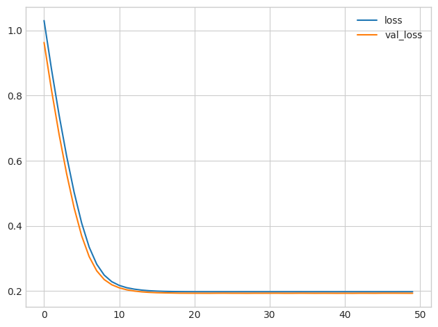

It's not uncommon for the curves to follow a "hockey stick" pattern like you see here. This makes the final part of training hard to see, so let's start at epoch 10 instead:

曲线遵循曲棍球棒模式并不罕见，就像您在此处看到的那样。 这使得训练的最后部分很难看到，所以让我们从第 10 轮开始：

# Start the plot at epoch 10
history_df.loc[10:, ['loss', 'val_loss']].plot()
print("Minimum Validation Loss: {:0.4f}".format(history_df['val_loss'].min()));

Minimum Validation Loss: 0.1929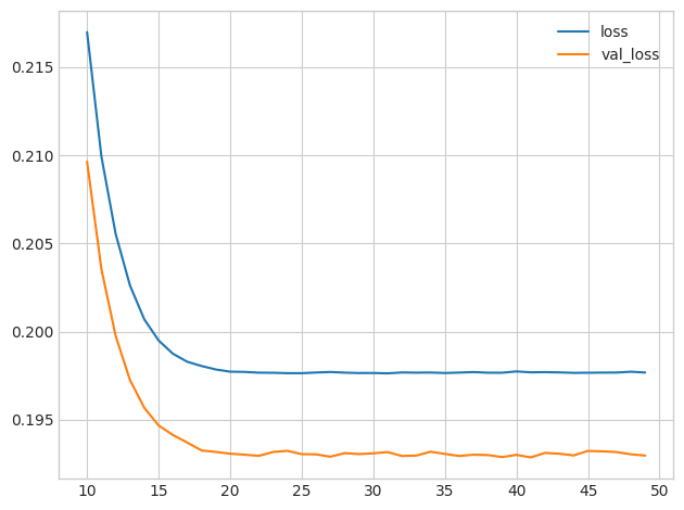

1) Evaluate Baseline

1) 评估基线

What do you think? Would you say this model is underfitting, overfitting, just right?

你怎么认为？ 你会说这个模型欠拟合、过拟合、恰到好处吗？

# View the solution (Run this cell to receive credit!)
q_1.check()

Correct:

The gap between these curves is quite small and the validation loss never increases, so it's more likely that the network is underfitting than overfitting. It would be worth experimenting with more capacity to see if that's the case.

这些曲线之间的差距非常小，并且验证损失永远不会增加，因此网络更有可能欠拟合而不是过拟合。 值得尝试更多的容量来看看情况是否如此。

Now let's add some capacity to our network. We'll add three hidden layers with 128 units each. Run the next cell to train the network and see the learning curves.

现在让我们为我们的网络添加一些容量。 我们将添加三个隐藏层，每个隐藏层有 128 个单元。 运行下一个单元来训练网络并查看学习曲线。

model = keras.Sequential([
    layers.Dense(128, activation='relu', input_shape=input_shape),
    layers.Dense(64, activation='relu'),
    layers.Dense(1)
])
model.compile(
    optimizer='adam',
    loss='mae',
)
history = model.fit(
    X_train, y_train,
    validation_data=(X_valid, y_valid),
    batch_size=512,
    epochs=50,
    verbose=False,
)
history_df = pd.DataFrame(history.history)
history_df.loc[:, ['loss', 'val_loss']].plot()
print("Minimum Validation Loss: {:0.4f}".format(history_df['val_loss'].min()));

Minimum Validation Loss: 0.1909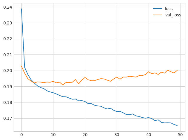

2) Add Capacity

2) 增加容量

What is your evaluation of these curves? Underfitting, overfitting, just right?

您对这些曲线有何评价？ 欠拟合、过拟合，刚刚好？

# View the solution (Run this cell to receive credit!)
q_2.check()

Correct:

Now the validation loss begins to rise very early, while the training loss continues to decrease. This indicates that the network has begun to overfit. At this point, we would need to try something to prevent it, either by reducing the number of units or through a method like early stopping. (We'll see another in the next lesson!)

现在验证损失很早就开始上升，而训练损失则持续下降。 这表明网络已经开始过拟合。 此时，我们需要尝试一些方法来防止它，要么通过减少单元数量，要么通过提前停止等方法。 （我们将在下一课中看到另一个！）

3) Define Early Stopping Callback

3) 定义提前停止回调

Now define an early stopping callback that waits 5 epochs (patience') for a change in validation loss of at least 0.001 (min_delta) and keeps the weights with the best loss (restore_best_weights).

现在定义一个提前停止回调，等待 5 个周期（patience），以等待验证损失至少达到0.001（min_delta）的变化，并保持权重具有最佳损失（restore_best_weights）。

from tensorflow.keras import callbacks

# YOUR CODE HERE: define an early stopping callback
# early_stopping = ____
early_stopping=callbacks.EarlyStopping(
    min_delta=0.001,
    patience=5,
    restore_best_weights=True,
)

# Check your answer
q_3.check()

Correct

# Lines below will give you a hint or solution code
#q_3.hint()
q_3.solution()

Solution:

early_stopping = callbacks.EarlyStopping(
    patience=5,
    min_delta=0.001,
    restore_best_weights=True,
)

Now run this cell to train the model and get the learning curves. Notice the callbacks argument in model.fit.

现在运行该单元来训练模型并获取学习曲线。 请注意model.fit中的callbacks参数。

model = keras.Sequential([
    layers.Dense(128, activation='relu', input_shape=input_shape),
    layers.Dense(64, activation='relu'),    
    layers.Dense(1)
])
model.compile(
    optimizer='adam',
    loss='mae',
)
history = model.fit(
    X_train, y_train,
    validation_data=(X_valid, y_valid),
    batch_size=512,
    epochs=50,
    callbacks=[early_stopping]
)
history_df = pd.DataFrame(history.history)
history_df.loc[:, ['loss', 'val_loss']].plot()
print("Minimum Validation Loss: {:0.4f}".format(history_df['val_loss'].min()));

Epoch 1/50
49/49 [==============================] - 1s 6ms/step - loss: 0.2685 - val_loss: 0.2070
Epoch 2/50
49/49 [==============================] - 0s 4ms/step - loss: 0.2043 - val_loss: 0.1988
Epoch 3/50
49/49 [==============================] - 0s 4ms/step - loss: 0.1988 - val_loss: 0.1958
Epoch 4/50
49/49 [==============================] - 0s 5ms/step - loss: 0.1953 - val_loss: 0.1948
Epoch 5/50
49/49 [==============================] - 0s 4ms/step - loss: 0.1932 - val_loss: 0.1945
Epoch 6/50
49/49 [==============================] - 0s 5ms/step - loss: 0.1918 - val_loss: 0.1933
Epoch 7/50
49/49 [==============================] - 0s 4ms/step - loss: 0.1897 - val_loss: 0.1935
Epoch 8/50
49/49 [==============================] - 0s 4ms/step - loss: 0.1886 - val_loss: 0.1933
Epoch 9/50
49/49 [==============================] - 0s 5ms/step - loss: 0.1879 - val_loss: 0.1928
Epoch 10/50
49/49 [==============================] - 0s 4ms/step - loss: 0.1861 - val_loss: 0.1942
Epoch 11/50
49/49 [==============================] - 0s 4ms/step - loss: 0.1860 - val_loss: 0.1932
Minimum Validation Loss: 0.1928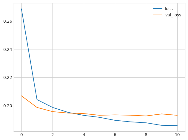

4) Train and Interpret

4) 训练和解释

Was this an improvement compared to training without early stopping?

与没有提前停止的训练相比，这是否有所改进？

# View the solution (Run this cell to receive credit!)
q_4.check()

Correct:

The early stopping callback did stop the training once the network began overfitting. Moreover, by including restore_best_weights we still get to keep the model where validation loss was lowest.

一旦网络开始过度拟合，提前停止的回调就会停止训练。 此外，通过包含restore_best_weights，我们仍然可以保持验证损失最低的模型。

If you like, try experimenting with patience and min_delta to see what difference it might make.

如果您愿意，请尝试不同的patience和min_delta，看看它会产生什么不同。

Keep Going

继续前进

Move on to learn about a couple of special layers: batch normalization and dropout.

继续了解几个特殊层：批量标准化和丢弃。