This notebook is an exercise in the Computer Vision course. You can reference the tutorial at this link.
Introduction
介绍
In these exercises, you'll conclude the feature extraction begun in Exercise 2, explore how invariance is created by maximum pooling, and then look at a different kind of pooling: average pooling.
在这些练习中,您将完成练习 2 中开始的特征提取,探索最大池化如何产生不变性,然后研究另一种池化:平均池化。
Run the cell below to set everything up.
运行下面的单元格以设置所有内容。
# Setup feedback system
from learntools.core import binder
binder.bind(globals())
from learntools.computer_vision.ex3 import *

import numpy as np
import tensorflow as tf
import matplotlib.pyplot as plt
from matplotlib import gridspec
import learntools.computer_vision.visiontools as visiontools

plt.rc('figure', autolayout=True)
plt.rc('axes', labelweight='bold', labelsize='large',
       titleweight='bold', titlesize=18, titlepad=10)
plt.rc('image', cmap='magma')
2024-08-09 09:03:54.769388: E external/local_xla/xla/stream_executor/cuda/cuda_dnn.cc:9261] Unable to register cuDNN factory: Attempting to register factory for plugin cuDNN when one has already been registered
2024-08-09 09:03:54.769463: E external/local_xla/xla/stream_executor/cuda/cuda_fft.cc:607] Unable to register cuFFT factory: Attempting to register factory for plugin cuFFT when one has already been registered
2024-08-09 09:03:54.771428: E external/local_xla/xla/stream_executor/cuda/cuda_blas.cc:1515] Unable to register cuBLAS factory: Attempting to register factory for plugin cuBLAS when one has already been registeredRun this cell to get back to where you left off in the previous lesson. We'll use a predefined kernel this time.
运行此单元可返回上一课中您离开的位置。这次我们将使用预定义内核。
# Read image
image_path = '../input/computer-vision-resources/car_illus.jpg'
image = tf.io.read_file(image_path)
image = tf.io.decode_jpeg(image, channels=1)
image = tf.image.resize(image, size=[400, 400])

# Embossing kernel
kernel = tf.constant([
    [-2, -1, 0],
    [-1, 1, 1],
    [0, 1, 2],
])

# Reformat for batch compatibility.
image = tf.image.convert_image_dtype(image, dtype=tf.float32)
image = tf.expand_dims(image, axis=0)
kernel = tf.reshape(kernel, [*kernel.shape, 1, 1])
kernel = tf.cast(kernel, dtype=tf.float32)

image_filter = tf.nn.conv2d(
    input=image,
    filters=kernel,
    strides=1,
    padding='VALID',
)

image_detect = tf.nn.relu(image_filter)

# Show what we have so far
plt.figure(figsize=(12, 6))
plt.subplot(131)
plt.imshow(tf.squeeze(image), cmap='gray')
plt.axis('off')
plt.title('Input')
plt.subplot(132)
plt.imshow(tf.squeeze(image_filter))
plt.axis('off')
plt.title('Filter')
plt.subplot(133)
plt.imshow(tf.squeeze(image_detect))
plt.axis('off')
plt.title('Detect')
plt.show();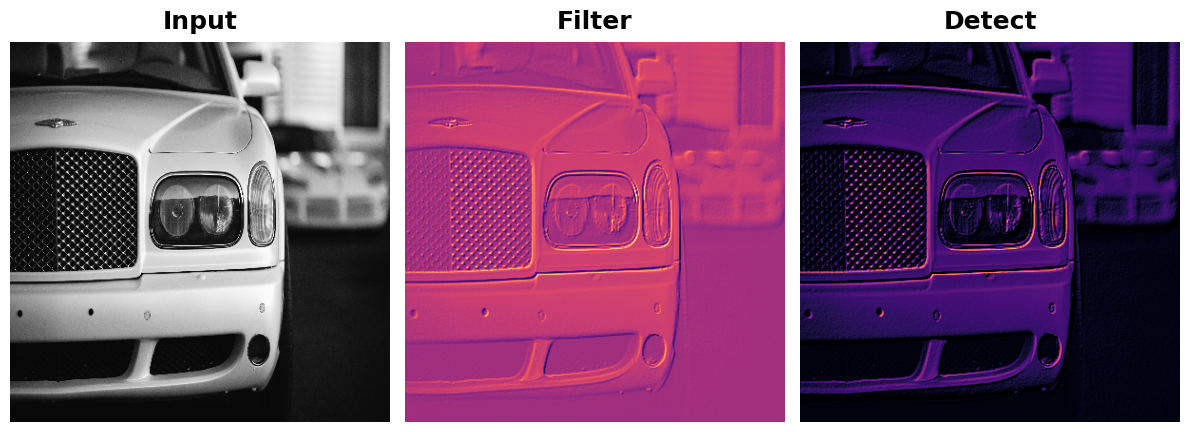
1) Apply Pooling to Condense
1) 应用池化来压缩
For for the last step in the sequence, apply maximum pooling using a $2 \times 2$ pooling window. You can copy this code to get started:
对于序列中的最后一步,使用 $2 \times 2$ 池化窗口应用最大池化。您可以复制此代码以开始使用:
image_condense = tf.nn.pool(
    input=image_detect,
    window_shape=____,
    pooling_type=____,
    strides=(2, 2),
    padding='SAME',
)
# YOUR CODE HERE
# image_condense = ____
image_condense = tf.nn.pool(
input=image_detect,
window_shape=(2, 2),
pooling_type='MAX',
strides=(2, 2),
padding='SAME',
)
# Check your answer
q_1.check()Correct
# Lines below will give you a hint or solution code
#q_1.hint()
q_1.solution()
Solution:
image_condense = tf.nn.pool(
    input=image_detect,
    window_shape=(2, 2),
    pooling_type='MAX',
    strides=(2, 2),
    padding='SAME',
)
Run the next cell to see what maximum pooling did to the feature!
运行下一个单元来查看最大池化对该特征做了什么!
plt.figure(figsize=(8, 6))
plt.subplot(121)
plt.imshow(tf.squeeze(image_detect))
plt.axis('off')
plt.title("Detect (ReLU)")
plt.subplot(122)
plt.imshow(tf.squeeze(image_condense))
plt.axis('off')
plt.title("Condense (MaxPool)")
plt.show();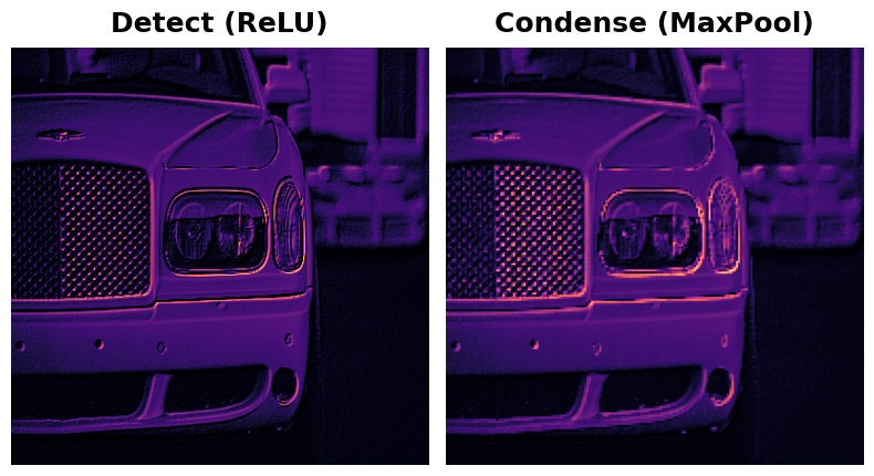
We learned about how MaxPool2D layers give a convolutional network the property of translation invariance over small distances. In this exercise, you'll have a chance to observe this in action.
我们了解了 MaxPool2D 层如何使卷积网络在短距离上具有 平移不变性 的特性。在本练习中,您将有机会观察这一特性的实际应用。
This next code cell will randomly apply a small shift to a circle and then condense the image several times with maximum pooling. Run the cell once and make note of the image that results at the end.
下一个代码单元将随机对圆圈应用小幅移位,然后使用最大池化多次压缩图像。运行该单元一次并记下最后生成的图像。
REPEATS = 4
SIZE = [64, 64]

# Create a randomly shifted circle
image = visiontools.circle(SIZE, r_shrink=4, val=1)
image = tf.expand_dims(image, axis=-1)
image = visiontools.random_transform(image, jitter=3, fill_method='replicate')
image = tf.squeeze(image)

plt.figure(figsize=(16, 4))
plt.subplot(1, REPEATS+1, 1)
plt.imshow(image, vmin=0, vmax=1)
plt.title("Original\nShape: {}x{}".format(image.shape[0], image.shape[1]))
plt.axis('off')

# Now condense with maximum pooling several times
for i in range(REPEATS):
    ax = plt.subplot(1, REPEATS+1, i+2)
    image = tf.reshape(image, [1, *image.shape, 1])
    image = tf.nn.pool(image, window_shape=(2,2), strides=(2, 2), padding='SAME', pooling_type='MAX')
    image = tf.squeeze(image)
    plt.imshow(image, vmin=0, vmax=1)
    plt.title("MaxPool {}\nShape: {}x{}".format(i+1, image.shape[0], image.shape[1]))
    plt.axis('off')
/tmp/__autograph_generated_filerc3mm1n8.py:62: SyntaxWarning: "is" with a literal. Did you mean "=="?
ag__.if_stmt(ag__.ld(fill_method) is 'reflect', if_body, else_body, get_state, set_state, ('i', 'j'), 2)
/tmp/__autograph_generated_filerc3mm1n8.py:63: SyntaxWarning: "is" with a literal. Did you mean "=="?
ag__.if_stmt(ag__.ld(fill_method) is 'replicate', if_body_1, else_body_1, get_state_1, set_state_1, ('i', 'j'), 2)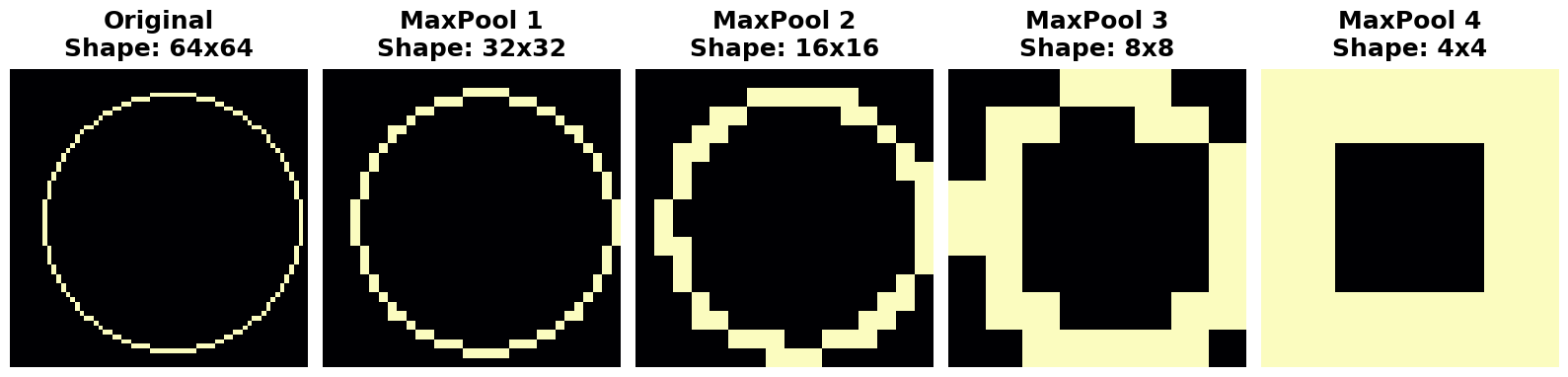
2) Explore Invariance
2) 探索不变性
Suppose you had made a small shift in a different direction -- what effect would you expect that have on the resulting image? Try running the cell a few more times, if you like, to get a new random shift.
假设你在不同方向上做了一点小调整——你认为这会对最终图像产生什么影响?如果愿意,可以尝试多运行几次单元,以获得新的随机调整。
# View the solution (Run this code cell to receive credit!)
q_2.solution()
Solution: In the tutorial, we talked about how maximum pooling creates translation invariance over small distances. This means that we would expect small shifts to disappear after repeated maximum pooling. If you run the cell multiple times, you can see the resulting image is always the same; the pooling operation destroys those small translations.
解决方案:在本教程中,我们讨论了最大池化如何在小距离上创建平移不变性。这意味着我们预计在重复最大池化之后,小的偏移会消失。如果多次运行该单元,您会发现生成的图像始终相同;池化操作会破坏那些小的平移。
Global Average Pooling
全局平均池化
We mentioned in the previous exercise that average pooling has largely been superceeded by maximum pooling within the convolutional base. There is, however, a kind of average pooling that is still widely used in the head of a convnet. This is global average pooling. A GlobalAvgPool2D layer is often used as an alternative to some or all of the hidden Dense layers in the head of the network, like so:
我们在上一个练习中提到,卷积基础中的平均池化已基本被最大池化所取代。然而,有一种平均池化仍然在卷积网络的头部中广泛使用。这就是全局平均池化。GlobalAvgPool2D 层通常用作网络头部中部分或全部隐藏的Dense 层的替代,如下所示:
model = keras.Sequential([
    pretrained_base,
    layers.GlobalAvgPool2D(),
    layers.Dense(1, activation='sigmoid'),
])
What is this layer doing? Notice that we no longer have the Flatten layer that usually comes after the base to transform the 2D feature data to 1D data needed by the classifier. Now the GlobalAvgPool2D layer is serving this function. But, instead of "unstacking" the feature (like Flatten), it simply replaces the entire feature map with its average value. Though very destructive, it often works quite well and has the advantage of reducing the number of parameters in the model.
这一层在做什么?请注意,我们不再有通常在基础层之后出现的Flatten层,用于将 2D 特征数据转换为分类器所需的 1D 数据。现在,GlobalAvgPool2D层正在提供此功能。但是,它不是拆分特征(如Flatten),而是用其平均值替换整个特征图。虽然破坏性很大,但它通常效果很好,并且具有减少模型中参数数量的优势。
Let's look at what GlobalAvgPool2D does on some randomly generated feature maps. This will help us to understand how it can "flatten" the stack of feature maps produced by the base.
让我们看看GlobalAvgPool2D在一些随机生成的特征图上做了什么。这将有助于我们理解它如何展平基础层生成的特征图堆栈。
Run this next cell a few times until you get a feel for how this new layer works.
运行下一个单元几次,直到您了解这个新层的工作原理。
feature_maps = [visiontools.random_map([5, 5], scale=0.1, decay_power=4) for _ in range(8)]

gs = gridspec.GridSpec(1, 8, wspace=0.01, hspace=0.01)
plt.figure(figsize=(18, 2))
for i, feature_map in enumerate(feature_maps):
    plt.subplot(gs[i])
    plt.imshow(feature_map, vmin=0, vmax=1)
    plt.axis('off')
plt.suptitle('Feature Maps', size=18, weight='bold', y=1.1)
plt.show()

# reformat for TensorFlow
feature_maps_tf = [tf.reshape(feature_map, [1, *feature_map.shape, 1])
                   for feature_map in feature_maps]

global_avg_pool = tf.keras.layers.GlobalAvgPool2D()
pooled_maps = [global_avg_pool(feature_map) for feature_map in feature_maps_tf]
img = np.array(pooled_maps)[:,:,0].T

plt.imshow(img, vmin=0, vmax=1)
plt.axis('off')
plt.title('Pooled Feature Maps')
plt.show();
/opt/conda/lib/python3.10/site-packages/IPython/core/pylabtools.py:152: UserWarning: This figure includes Axes that are not compatible with tight_layout, so results might be incorrect.
fig.canvas.print_figure(bytes_io, **kw)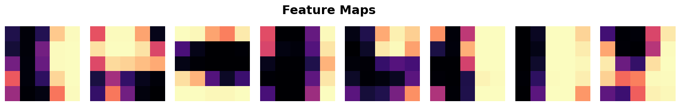

Since each of the $5 \times 5$ feature maps was reduced to a single value, global pooling reduced the number of parameters needed to represent these features by a factor of 25 -- a substantial savings!
由于每个 $5 \times 5$ 特征图都缩减为单个值,因此全局池化将表示这些特征所需的参数数量减少了 25 倍——节省了大量资源!
Now we'll move on to understanding the pooled features.
现在我们将继续了解池化特征。
After we've pooled the features into just a single value, does the head still have enough information to determine a class? This part of the exercise will investigate that question.
在我们将特征池化为单个值后,头部是否仍有足够的信息来确定类别?本部分练习将调查这个问题。
Let's pass some images from our Car or Truck dataset through VGG16 and examine the features that result after pooling. First run this cell to define the model and load the dataset.
让我们通过 VGG16 传递一些来自 Car or Truck 数据集的图像,并检查池化后产生的特征。首先运行此单元以定义模型并加载数据集。
from tensorflow import keras
from tensorflow.keras import layers
from tensorflow.keras.preprocessing import image_dataset_from_directory

# Load VGG16
pretrained_base = tf.keras.models.load_model(
    '../input/cv-course-models/cv-course-models/vgg16-pretrained-base',
)

model = keras.Sequential([
    pretrained_base,
    # Attach a global average pooling layer after the base
    layers.GlobalAvgPool2D(),
])

# Load dataset
ds = image_dataset_from_directory(
    '../input/car-or-truck/train',
    labels='inferred',
    label_mode='binary',
    image_size=[128, 128],
    interpolation='nearest',
    batch_size=1,
    shuffle=True,
)

ds_iter = iter(ds)
Found 5117 files belonging to 2 classes.Notice how we've attached a GlobalAvgPool2D layer after the pretrained VGG16 base. Ordinarily, VGG16 will produce 512 feature maps for each image. The GlobalAvgPool2D layer reduces each of these to a single value, an "average pixel", if you like.
请注意,我们在预训练的 VGG16 基础层之后附加了一个 GlobalAvgPool2D 层。通常,VGG16 将为每个图像生成 512 个特征图。如果您愿意的话,GlobalAvgPool2D 层将每个特征图简化为一个值,即“平均像素”。
This next cell will run an image from the Car or Truck dataset through VGG16 and show you the 512 average pixels created by GlobalAvgPool2D. Run the cell a few times and observe the pixels produced by cars versus the pixels produced by trucks.
下一个单元将通过 VGG16 运行来自 Car or Truck 数据集的图像,并向您显示由 GlobalAvgPool2D 创建的 512 个平均像素。运行该单元几次,并观察汽车产生的像素与卡车产生的像素。
car = next(ds_iter)

car_tf = tf.image.resize(car[0], size=[128, 128])
car_features = model(car_tf)
car_features = tf.reshape(car_features, shape=(16, 32))
label = int(tf.squeeze(car[1]).numpy())

plt.figure(figsize=(8, 4))
plt.subplot(121)
plt.imshow(tf.squeeze(car[0]))
plt.axis('off')
plt.title(["Car", "Truck"][label])
plt.subplot(122)
plt.imshow(car_features)
plt.title('Pooled Feature Maps')
plt.axis('off')
plt.show();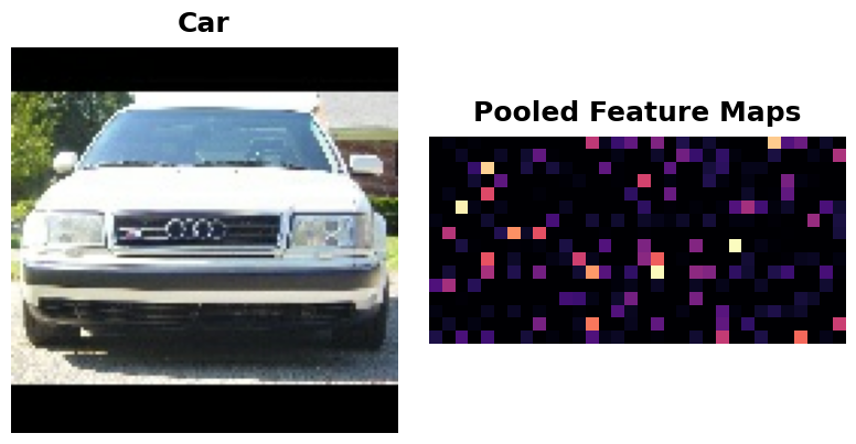
3) Understand the Pooled Features
3) 了解池化特征
What do you see? Are the pooled features for cars and trucks different enough to tell them apart? How would you interpret these pooled values? How could this help the classification? After you've thought about it, run the next cell for an answer. (Or see a hint first!)
您看到了什么?汽车和卡车的池化特征是否足够不同以区分它们?您如何解释这些池化值?这对分类有何帮助?思考过后,运行下一个单元以找到答案。(或者先看提示!)
# View the solution (Run this code cell to receive credit!)
q_3.check()
Correct:
The VGG16 base produces 512 feature maps. We can think of each feature map as representing some high-level visual feature in the original image -- maybe a wheel or window. Pooling a map gives us a single number, which we could think of as a score for that feature: large if the feature is present, small if it is absent. Cars tend to score high with one set of features, and Trucks score high with another. Now, instead of trying to map raw features to classes, the head only has to work with these scores that GlobalAvgPool2D produced, a much easier problem for it to solve.
VGG16 基础生成 512 个特征图。我们可以将每个特征图视为原始图像中的一些高级视觉特征 - 可能是车轮或窗户。池化图会给我们一个数字,我们可以将其视为该特征的分数:如果该特征存在,则分数大,如果不存在,则分数小。汽车往往在一组特征中得分高,而卡车在另一组特征中得分高。现在,头部不必尝试将原始特征映射到类别,只需使用 GlobalAvgPool2D 生成的这些分数,这对它来说是一个更容易解决的问题。
# Line below will give you a hint
q_3.hint()
Hint: VGG16 creates 512 features maps from an image, which might represent something like a wheel or a window. Each square in Pooled Feature Maps represents a feature. What would a large value for a feature mean?
Global average pooling is often used in modern convnets. One big advantage is that it greatly reduces the number of parameters in a model, while still telling you if some feature was present in an image or not -- which for classification is usually all that matters. If you're creating a convolutional classifier it's worth trying out!
全局平均池化通常用于现代卷积网络。一个很大的优点是它大大减少了模型中的参数数量,同时仍能告诉您图像中是否存在某些特征——这对于分类来说通常是最重要的。如果您正在创建卷积分类器,它值得一试!
Conclusion
结论
In this lesson we explored the final operation in the feature extraction process: condensing with maximum pooling. Pooling is one of the essential features of convolutional networks and helps provide them with some of their characteristic advantages: efficiency with visual data, reduced parameter size compared to dense networks, translation invariance. We've seen that it's used not only in the base during feature extraction, but also can be used in the head during classification. Understanding it is essential to a full understanding of convnets.
在本课中,我们探讨了特征提取过程中的最后一个操作:使用 最大池化 进行 压缩。池化是卷积网络的基本特征之一,有助于为它们提供一些特征优势:视觉数据的效率、与密集网络相比参数大小减小、平移不变性。我们已经看到它不仅在特征提取期间用于基,还可以在分类期间用于头部。理解它对于全面理解卷积网络至关重要。
Keep Going
继续
In the next lesson, we'll conclude our discussion of the feature extraction operations with sliding windows, the typical way of describing how the convolution and pooling operations scan over an image. We'll describe here the final two parameters in the Conv2D and MaxPool2D layers: strides and padding. Check it out now!
在下一课中,我们将结束对使用 滑动窗口 的特征提取操作的讨论,这是描述卷积和池化操作如何扫描图像的典型方式。我们将在这里描述 Conv2D 和 MaxPool2D 层中的最后两个参数:strides 和 padding。立即查看!