This notebook is an exercise in the Computer Vision course. You can reference the tutorial at this link.

---

Introduction

介绍

In these exercises, you'll build a custom convnet with performance competitive to the VGG16 model from Lesson 1.

在这些练习中，您将构建一个自定义卷积网络，其性能可与第 1 课中的 VGG16 模型相媲美。

Get started by running the code cell below.

通过运行下面的代码单元开始。

# Setup feedback system
from learntools.core import binder
binder.bind(globals())
from learntools.computer_vision.ex5 import *

# Imports
import os, warnings
import matplotlib.pyplot as plt
from matplotlib import gridspec

import numpy as np
import tensorflow as tf
from tensorflow.keras.preprocessing import image_dataset_from_directory

# Reproducability
def set_seed(seed=31415):
    np.random.seed(seed)
    tf.random.set_seed(seed)
    os.environ['PYTHONHASHSEED'] = str(seed)
    os.environ['TF_DETERMINISTIC_OPS'] = '1'
set_seed()

# Set Matplotlib defaults
plt.rc('figure', autolayout=True)
plt.rc('axes', labelweight='bold', labelsize='large',
       titleweight='bold', titlesize=18, titlepad=10)
plt.rc('image', cmap='magma')
warnings.filterwarnings("ignore") # to clean up output cells

# Load training and validation sets
ds_train_ = image_dataset_from_directory(
    '../input/car-or-truck/train',
    labels='inferred',
    label_mode='binary',
    image_size=[128, 128],
    interpolation='nearest',
    batch_size=64,
    shuffle=True,
)
ds_valid_ = image_dataset_from_directory(
    '../input/car-or-truck/valid',
    labels='inferred',
    label_mode='binary',
    image_size=[128, 128],
    interpolation='nearest',
    batch_size=64,
    shuffle=False,
)

# Data Pipeline
def convert_to_float(image, label):
    image = tf.image.convert_image_dtype(image, dtype=tf.float32)
    return image, label

AUTOTUNE = tf.data.experimental.AUTOTUNE
ds_train = (
    ds_train_
    .map(convert_to_float)
    .cache()
    .prefetch(buffer_size=AUTOTUNE)
)
ds_valid = (
    ds_valid_
    .map(convert_to_float)
    .cache()
    .prefetch(buffer_size=AUTOTUNE)
)

2024-08-29 08:16:03.293281: E external/local_xla/xla/stream_executor/cuda/cuda_dnn.cc:9261] Unable to register cuDNN factory: Attempting to register factory for plugin cuDNN when one has already been registered
2024-08-29 08:16:03.293344: E external/local_xla/xla/stream_executor/cuda/cuda_fft.cc:607] Unable to register cuFFT factory: Attempting to register factory for plugin cuFFT when one has already been registered
2024-08-29 08:16:03.295008: E external/local_xla/xla/stream_executor/cuda/cuda_blas.cc:1515] Unable to register cuBLAS factory: Attempting to register factory for plugin cuBLAS when one has already been registered

Found 5117 files belonging to 2 classes.
Found 5051 files belonging to 2 classes.

Design a Convnet

设计一个卷积网络

Let's design a convolutional network with a block architecture like we saw in the tutorial. The model from the example had three blocks, each with a single convolutional layer. Its performance on the "Car or Truck" problem was okay, but far from what the pretrained VGG16 could achieve. It might be that our simple network lacks the ability to extract sufficiently complex features. We could try improving the model either by adding more blocks or by adding convolutions to the blocks we have.

让我们设计一个像教程中看到的块架构的卷积网络。示例中的模型有三个块，每个块都有一个卷积层。它在汽车或卡车问题上的表现还不错，但远不及预训练的 VGG16 所能达到的水平。可能是我们的简单网络缺乏提取足够复杂特征的能力。我们可以尝试通过添加更多块或向现有块添加卷积来改进模型。

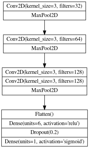
Let's go with the second approach. We'll keep the three block structure, but increase the number of Conv2D layer in the second block to two, and in the third block to three.

让我们采用第二种方法。我们将保留三个块结构，但将第二个块中的Conv2D层的数量增加到两个，将第三个块中的Conv2D层的数量增加到三个。

1) Define Model

1) 定义模型

Given the diagram above, complete the model by defining the layers of the third block.

根据上图，通过定义第三块的层来完成模型。

from tensorflow import keras
from tensorflow.keras import layers

model = keras.Sequential([
    # Block One
    layers.Conv2D(filters=32, kernel_size=3, activation='relu', padding='same',
                  input_shape=[128, 128, 3]),
    layers.MaxPool2D(),

    # Block Two
    layers.Conv2D(filters=64, kernel_size=3, activation='relu', padding='same'),
    layers.MaxPool2D(),

    # Block Three
    # YOUR CODE HERE
    # ____,
    layers.Conv2D(filters=128, kernel_size=3, activation='relu', padding='same'),
    layers.Conv2D(filters=128, kernel_size=3, activation='relu', padding='same'),
    layers.MaxPool2D(),

    # Head
    layers.Flatten(),
    layers.Dense(6, activation='relu'),
    layers.Dropout(0.2),
    layers.Dense(1, activation='sigmoid'),
])

# Check your answer
q_1.check()

Correct

# Lines below will give you a hint or solution code
#q_1.hint()
#q_1.solution()

2) Compile

2) 编译

To prepare for training, compile the model with an appropriate loss and accuracy metric for the "Car or Truck" dataset.

为准备训练，请使用适合“汽车或卡车”数据集的损失和准确度指标编译模型。

model.compile(
    optimizer=tf.keras.optimizers.Adam(epsilon=0.01),
    # YOUR CODE HERE: Add loss and metric
    loss='binary_crossentropy',
    metrics=['binary_accuracy']
)

# Check your answer
q_2.check()

Correct

model.compile(
    optimizer=tf.keras.optimizers.Adam(epsilon=0.01),
    loss='binary_crossentropy',
    metrics=['binary_accuracy'],
)
q_2.assert_check_passed()

Correct

# Lines below will give you a hint or solution code
#q_2.hint()
#q_2.solution()

Finally, let's test the performance of this new model. First run this cell to fit the model to the training set.

最后，让我们测试一下这个新模型的性能。首先运行此单元，使模型适合训练集。

history = model.fit(
    ds_train,
    validation_data=ds_valid,
    epochs=50,
    verbose=False,
)

WARNING: All log messages before absl::InitializeLog() is called are written to STDERR
I0000 00:00:1724919382.543470    1219 device_compiler.h:186] Compiled cluster using XLA!  This line is logged at most once for the lifetime of the process.

And now run the cell below to plot the loss and metric curves for this training run.

import pandas as pd
history_frame = pd.DataFrame(history.history)
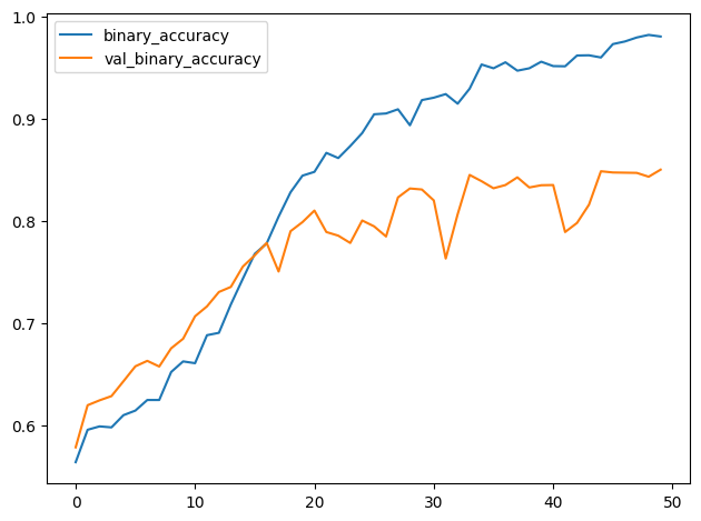
history_frame.loc[:, ['loss', 'val_loss']].plot()
history_frame.loc[:, ['binary_accuracy', 'val_binary_accuracy']].plot();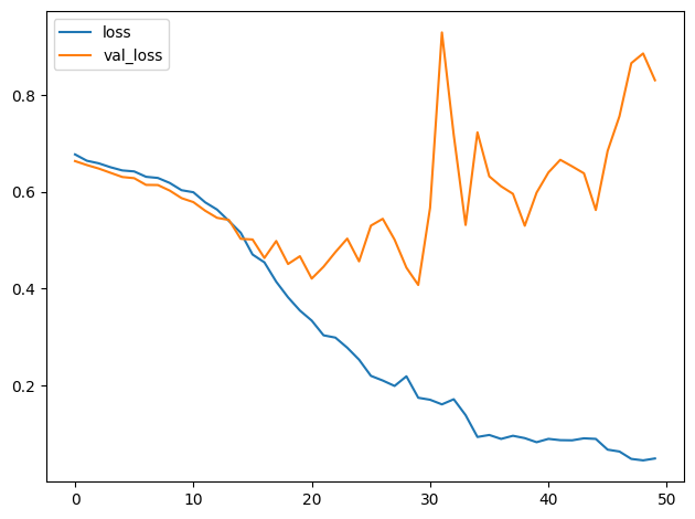

3) Train the Model

3) 训练模型

How would you interpret these training curves? Did this model improve upon the model from the tutorial?

您如何解释这些训练曲线？该模型是否比教程中的模型有所改进？

# View the solution (Run this code cell to receive credit!)
q_3.check()

Correct:

The learning curves for the model from the tutorial diverged fairly rapidly. This would indicate that it was prone to overfitting and in need of some regularization. The additional layer in our new model would make it even more prone to overfitting. However, adding some regularization with the Dropout layer helped prevent this. These changes improved the validation accuracy of the model by several points.

教程中模型的学习曲线分化得相当快。这表明它容易过度拟合，需要一些正则化。我们新模型中的附加层会使其更容易过度拟合。但是，使用 Dropout 层添加一些正则化有助于防止这种情况。这些变化将模型的验证准确率提高了几个百分点。

Conclusion

结论

These exercises showed you how to design a custom convolutional network to solve a specific classification problem. Though most models these days will be built on top of a pretrained base, it certain circumstances a smaller custom convnet might still be preferable -- such as with a smaller or unusual dataset or when computing resources are very limited. As you saw here, for certain problems they can perform just as well as a pretrained model.

这些练习向您展示了如何设计自定义卷积网络来解决特定的分类问题。虽然如今大多数模型都是在预训练的基础上构建的，但在某些情况下，较小的自定义卷积网络可能仍然是首选——例如，数据集较小或不寻常，或者计算资源非常有限。正如您在此处看到的，对于某些问题，它们的表现与预训练模型一样好。

Keep Going

继续

Continue on to Lesson 6, where you'll learn a widely-used technique that can give a boost to your training data: data augmentation.

继续学习 第 6 课，您将在其中学习一种可以增强训练数据的广泛使用的技术：数据增强。

---