This notebook is an exercise in the Machine Learning Explainability course. You can reference the tutorial at this link.
Set Up
设置
Today you will create partial dependence plots and practice building insights with data from the Taxi Fare Prediction competition.
今天,您将创建部分依赖关系图,并练习使用来自 出租车费预测 竞赛的数据来阐述问题。
We have again provided code to do the basic loading, review and model-building. Run the cell below to set everything up:
我们再次提供了代码来执行基本的加载、审查和模型构建。运行下面的单元格以设置所有内容:
import pandas as pd
from sklearn.ensemble import RandomForestRegressor
from sklearn.linear_model import LinearRegression
from sklearn.model_selection import train_test_split

# Environment Set-Up for feedback system.
from learntools.core import binder
binder.bind(globals())
from learntools.ml_explainability.ex3 import *
print("Setup Complete")

# Data manipulation code below here
data = pd.read_csv('../input/new-york-city-taxi-fare-prediction/train.csv', nrows=50000)

# Remove data with extreme outlier coordinates or negative fares
data = data.query('pickup_latitude > 40.7 and pickup_latitude < 40.8 and ' +
                  'dropoff_latitude > 40.7 and dropoff_latitude < 40.8 and ' +
                  'pickup_longitude > -74 and pickup_longitude < -73.9 and ' +
                  'dropoff_longitude > -74 and dropoff_longitude < -73.9 and ' +
                  'fare_amount > 0'
                  )

y = data.fare_amount

base_features = ['pickup_longitude',
                 'pickup_latitude',
                 'dropoff_longitude',
                 'dropoff_latitude']

X = data[base_features]

train_X, val_X, train_y, val_y = train_test_split(X, y, random_state=1)
first_model = RandomForestRegressor(n_estimators=30, random_state=1).fit(train_X, train_y)
print("Data sample:")
data.head()
Setup Complete
Data sample:| key | fare_amount | pickup_datetime | pickup_longitude | pickup_latitude | dropoff_longitude | dropoff_latitude | passenger_count | |
|---|---|---|---|---|---|---|---|---|
| 2 | 2011-08-18 00:35:00.00000049 | 5.7 | 2011-08-18 00:35:00 UTC | -73.982738 | 40.761270 | -73.991242 | 40.750562 | 2 |
| 3 | 2012-04-21 04:30:42.0000001 | 7.7 | 2012-04-21 04:30:42 UTC | -73.987130 | 40.733143 | -73.991567 | 40.758092 | 1 |
| 4 | 2010-03-09 07:51:00.000000135 | 5.3 | 2010-03-09 07:51:00 UTC | -73.968095 | 40.768008 | -73.956655 | 40.783762 | 1 |
| 6 | 2012-11-20 20:35:00.0000001 | 7.5 | 2012-11-20 20:35:00 UTC | -73.980002 | 40.751662 | -73.973802 | 40.764842 | 1 |
| 7 | 2012-01-04 17:22:00.00000081 | 16.5 | 2012-01-04 17:22:00 UTC | -73.951300 | 40.774138 | -73.990095 | 40.751048 | 1 |
data.describe()| fare_amount | pickup_longitude | pickup_latitude | dropoff_longitude | dropoff_latitude | passenger_count | |
|---|---|---|---|---|---|---|
| count | 31289.000000 | 31289.000000 | 31289.000000 | 31289.000000 | 31289.000000 | 31289.000000 |
| mean | 8.483093 | -73.976860 | 40.756917 | -73.975342 | 40.757473 | 1.656141 |
| std | 4.628164 | 0.014635 | 0.018170 | 0.015917 | 0.018661 | 1.284899 |
| min | 0.010000 | -73.999999 | 40.700013 | -73.999999 | 40.700020 | 0.000000 |
| 25% | 5.500000 | -73.988039 | 40.744947 | -73.987125 | 40.745922 | 1.000000 |
| 50% | 7.500000 | -73.979691 | 40.758027 | -73.978547 | 40.758559 | 1.000000 |
| 75% | 10.100000 | -73.967823 | 40.769580 | -73.966435 | 40.770427 | 2.000000 |
| max | 165.000000 | -73.900062 | 40.799952 | -73.900062 | 40.799999 | 6.000000 |
Question 1
问题 1
Here is the code to plot the partial dependence plot for pickup_longitude. Run the following cell without changes.
以下是绘制pickup_longitude部分依赖关系图的代码。运行以下单元格,无需更改。
from matplotlib import pyplot as plt
from sklearn.inspection import PartialDependenceDisplay

feat_name = 'pickup_longitude'
PartialDependenceDisplay.from_estimator(first_model, val_X, [feat_name])
plt.show()
Why does the partial dependence plot have this U-shape?
为什么部分依赖图有这种 U 形?
Does your explanation suggest what shape to expect in the partial dependence plots for the other features?
您的解释是否表明了其他特征的部分依赖图应有的形状?
Create all other partial plots in a for-loop below (copying the appropriate lines from the code above).
在下面的 for 循环中创建所有其他部分图(从上面的代码中复制相应的行)。
PartialDependenceDisplay.from_estimator(first_model, val_X, base_features)
plt.show()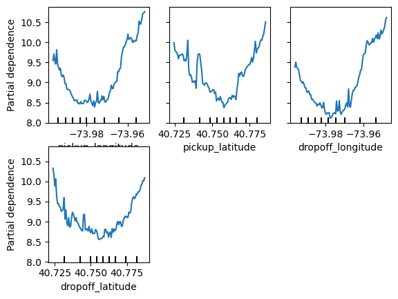
for feat_name in base_features:
    # ____
    PartialDependenceDisplay.from_estimator(first_model, val_X, [feat_name])
    plt.show()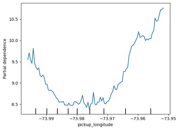
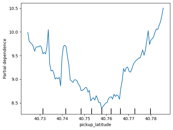
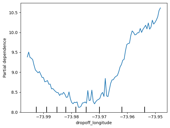
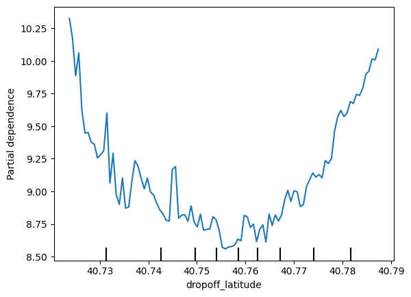
Do the shapes match your expectations for what shapes they would have? Can you explain the shape now that you've seen them?
这些形状符合你的预期吗?现在你已经看到它们了,你能解释一下它们的形状吗?
Uncomment the following line to check your intuition.
取消以下行的注释以检查你的直觉。
# Check your answer (Run this code cell to receive credit!)
q_1.solution()
Solution:
The code is
for feat_name in base_features:
    PartialDependenceDisplay.from_estimator(first_model, val_X, [feat_name])
    plt.show()
We have a sense from the permutation importance results that distance is the most important determinant of taxi fare.
This model didn't include distance measures (like absolute change in latitude or longitude) as features, so coordinate features (like pickup_longitude) capture the effect of distance.
Being picked up near the center of the longitude values lowers predicted fares on average, because it means shorter trips (on average).
For the same reason, we see the general U-shape in all our partial dependence plots.
我们从排列重要性结果中感觉到,距离是出租车费的最重要决定因素。
该模型未将距离度量(如纬度或经度的绝对变化)作为特征,因此坐标特征(如 pickup_longitude)可捕捉距离的影响。在经度值中心附近上车会降低平均预测费用,因为这意味着行程更短(平均而言)。
出于同样的原因,我们在所有部分依赖图中都看到了一般的 U 形。
Question 2
问题 2
Now you will run a 2D partial dependence plot. As a reminder, here is the code from the tutorial.
现在您将运行 2D 部分依赖图。提醒一下,这是本教程中的代码。
fig, ax = plt.subplots(figsize=(8, 6))
f_names = [('Goal Scored', 'Distance Covered (Kms)')]
PartialDependenceDisplay.from_estimator(tree_model, val_X, f_names, ax=ax)
plt.show()
Create a 2D plot for the features pickup_longitude and dropoff_longitude.
为特征pickup_longitude和dropoff_longitude创建一个二维图。
What do you expect it to look like?
你希望它看起来像什么?
fig, ax = plt.subplots(figsize=(8, 6))

# Add your code here
# ____
f_names = [('pickup_longitude', 'dropoff_longitude')]
PartialDependenceDisplay.from_estimator(first_model, val_X, f_names, ax=ax)
plt.show()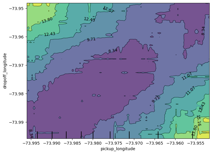
Uncomment the line below to see the solution and explanation for how one might reason about the plot shape.
取消注释下面这一行,以查看解决方案和如何推断绘图形状的解释。
# Check your answer (Run this code cell to receive credit!)
q_2.solution()
Solution:
You should expect the plot to have contours running along a diagonal. We see that to some extent, though there are interesting caveats.
We expect the diagonal contours because these are pairs of values where the pickup and dropoff longitudes are nearby, indicating shorter trips (controlling for other factors).
As you get further from the central diagonal, we should expect prices to increase as the distances between the pickup and dropoff longitudes also increase.
The surprising feature is that prices increase as you go further to the upper-right of this graph, even staying near that 45-degree line.
This could be worth further investigation, though the effect of moving to the upper right of this graph is small compared to moving away from that 45-degree line.
The code you need to create the desired plot is:
fig, ax = plt.subplots(figsize=(8, 6))
fnames = [('pickup_longitude', 'dropoff_longitude')]
disp = PartialDependenceDisplay.from_estimator(first_model, val_X, fnames, ax=ax)
plt.show()
您应该预期该图的轮廓线沿对角线延伸。我们在某种程度上看到了这一点,尽管也有一些有趣的警告。
我们预期对角线轮廓线,因为这些是上车点和下车点经度相近的值对,表示行程较短(控制其他因素)。
当您离中央对角线越来越远时,我们应该预期价格会随着上车点和下车点经度之间的距离增加而上涨。
令人惊讶的是,当您进一步向该图的右上方移动时,即使停留在 45 度线附近,价格也会上涨。
这可能值得进一步研究,尽管与远离 45 度线相比,向该图的右上方移动的影响很小。
Question 3
问题 3
Consider a ride starting at longitude -73.955 and ending at longitude -74. Using the graph from the last question, estimate how much money the rider would have saved if they'd started the ride at longitude -73.98 instead.
假设骑行从经度 -73.955 开始,到经度 -74 结束。使用上一个问题的图表,估算如果骑行者从经度 -73.98 开始骑行,可以节省多少钱。
# savings_from_shorter_trip = ____
savings_from_shorter_trip = first_model.predict(pd.DataFrame([[-73.955,train_X['pickup_latitude'].mean(),-74.,train_X['dropoff_latitude'].mean()]],columns=train_X.columns)) - first_model.predict(pd.DataFrame([[-73.98,train_X['pickup_latitude'].mean(),-74.,train_X['dropoff_latitude'].mean()]],columns=train_X.columns))
print(savings_from_shorter_trip)
# Check your answer
q_3.check()[6.748]Correct:
About 6. The price decreases from slightly less than 15 to slightly less than 9.
大概是6。价格从略低于15下降到略低于9。
For a solution or hint, uncomment the appropriate line below.
如需解决方案或提示,请取消注释下面相应的行。
q_3.hint()
# q_3.solution()
Hint: First find the vertical level corresponding to -74 dropoff longitude. Then read off the horizontal values you are switching between. Use the contour lines to orient yourself on what values you are near. You can round to the nearest integer rather than stressing about the exact cost to the nearest penny
提示:首先找到与 -74 下车经度相对应的垂直水平。然后读出您要切换的水平值。使用等高线来确定您附近的值。您可以四舍五入到最接近的整数,而不必担心精确到最接近的美分的费用。
Question 4
问题 4
In the PDP's you've seen so far, location features have primarily served as a proxy to capture distance traveled. In the permutation importance lessons, you added the features abs_lon_change and abs_lat_change as a more direct measure of distance.
在您目前看到的 PDP 中,位置特征主要用作捕获行进距离的替代。在排列重要性课程中,您添加了特征abs_lon_change和abs_lat_change作为更直接的距离测量。
Create these features again here. You only need to fill in the top two lines. Then run the following cell.
在此处再次创建这些特征。您只需填写前两行。然后运行以下单元格。
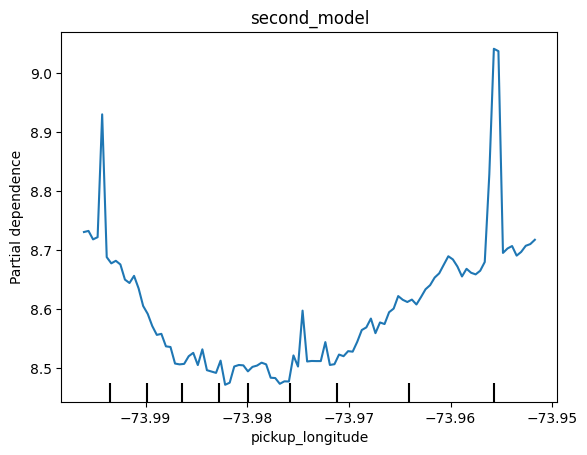
After you run it, identify the most important difference between this partial dependence plot and the one you got without absolute value features. The code to generate the PDP without absolute value features is at the top of this code cell.
运行后,确定此部分依赖图与您在没有绝对值特征的情况下得到的图之间的最重要差异。生成没有绝对值特征的 PDP 的代码位于此代码单元的顶部。
# This is the PDP for pickup_longitude without the absolute difference features. Included here to help compare it to the new PDP you create
feat_name = 'pickup_longitude'
PartialDependenceDisplay.from_estimator(first_model, val_X, [feat_name])
plt.title('first_model')
plt.show()

# Your code here
# create new features
# data['abs_lon_change'] = ____
# data['abs_lat_change'] = ____

data['abs_lon_change'] = abs(data['pickup_longitude'] - data['dropoff_longitude'])
data['abs_lat_change'] = abs(data['pickup_latitude'] - data['dropoff_latitude'])

features_2  = ['pickup_longitude',
               'pickup_latitude',
               'dropoff_longitude',
               'dropoff_latitude',
               'abs_lat_change',
               'abs_lon_change']

X = data[features_2]
new_train_X, new_val_X, new_train_y, new_val_y = train_test_split(X, y, random_state=1)
second_model = RandomForestRegressor(n_estimators=30, random_state=1).fit(new_train_X, new_train_y)

feat_name = 'pickup_longitude'
disp = PartialDependenceDisplay.from_estimator(second_model, new_val_X, [feat_name])
plt.title('second_model')
plt.show()

# Check your answer
q_4.check()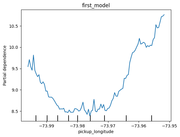
Correct:
The difference is that the partial dependence plot became smaller. Both plots have a lowest vertical value of 8.5. But, the highest vertical value in the top chart is around 10.7, and the highest vertical value in the bottom chart is below 9.1. In other words, once you control for absolute distance traveled, the pickup_longitude has a smaller impact on predictions.
# create new features
data['abs_lon_change'] = abs(data.dropoff_longitude - data.pickup_longitude)
data['abs_lat_change'] = abs(data.dropoff_latitude - data.pickup_latitude)
不同之处在于部分依赖图变小了。两个图的最低垂直值均为 8.5。但是,上图中的最高垂直值约为 10.7,而下图中的最高垂直值低于 9.1。换句话说,一旦控制了绝对行驶距离,pickup_longitude 对预测的影响就会变小。
Uncomment the line below to see a hint or the solution (including an explanation of the important differences between the plots).
取消注释下面这一行来查看提示或解决方案(包括对图表之间重要差异的解释)。
q_4.hint()
# q_4.solution()
Hint: Use the abs function when creating the abs_lat_change and abs_lon_change features. You don't need to change anything else.
提示:创建 abs_lat_change 和 abs_lon_change 特征时使用 abs 函数。您无需更改任何其他内容。
Question 5
问题 5
Consider a scenario where you have only 2 predictive features, which we will call feat_A and feat_B. Both features have minimum values of -1 and maximum values of 1. The partial dependence plot for feat_A increases steeply over its whole range, whereas the partial dependence plot for feature B increases at a slower rate (less steeply) over its whole range.
考虑这样一种情况,您只有 2 个预测特征,我们将其称为feat_A和feat_B。这两个特征的最小值均为 -1,最大值均为 1。feat_A的部分依赖图在其整个范围内急剧增加,而特征 B 的部分依赖图在其整个范围内以较慢的速度(不太陡峭)增加。
Does this guarantee that feat_A will have a higher permutation importance than feat_B. Why or why not?
这是否保证feat_A的排列重要性将高于feat_B。为什么或为什么不?
After you've thought about it, uncomment the line below for the solution.
考虑过后,取消注释下面的行以获得解决方案。
# Check your answer (Run this code cell to receive credit!)
q_5.solution()
Solution: No. This doesn't guarantee feat_a is more important. For example, feat_a could have a big effect in the cases where it varies, but could have a single value 99\% of the time. In that case, permuting feat_a wouldn't matter much, since most values would be unchanged.
不。这并不能保证 feat_a 更重要。例如,feat_a 在其变化的情况下可能会产生很大影响,但 99% 的时间可能只有一个值。在这种情况下,对 feat_a 进行排列并不重要,因为大多数值都不会改变。
Question 6
问题 6
The code cell below does the following:
下面的代码单元执行以下操作:
- Creates two features,
X1andX2, having random values in the range [-2, 2]. - 创建两个特征
X1和X2,其随机值在 [-2, 2] 范围内。 - Creates a target variable
y, which is always 1. - 创建目标变量
y,始终为 1。 - Trains a
RandomForestRegressormodel to predictygivenX1andX2. - 训练
RandomForestRegressor模型以在给定X1和X2的情况下预测y。 - Creates a PDP plot for
X1and a scatter plot ofX1vs.y. - 为
X1创建 PDP 图以及X1与y的散点图。
Do you have a prediction about what the PDP plot will look like? Run the cell to find out.
您对 PDP 图的外观有什么预测吗?运行该单元以找出答案。
Modify the initialization of y so that our PDP plot has a positive slope in the range [-1,1], and a negative slope everywhere else. (Note: you should only modify the creation of y, leaving X1, X2, and my_model unchanged.)
修改 y 的初始化,以便我们的 PDP 图在 [-1,1] 范围内具有正斜率,在其他地方具有负斜率。(注意:您应该只修改 y 的创建,而保持 X1、X2 和 my_model 不变。)
import numpy as np
from numpy.random import rand

n_samples = 20000

# Create array holding predictive feature
X1 = 4 * rand(n_samples) - 2
X2 = 4 * rand(n_samples) - 2

# Your code here
# Create y. you should have X1 and X2 in the expression for y
# y = np.ones(n_samples)
y = -2 * X1 * (X1<-1) + X1 - 2 * X1 * (X1>1) - X2

# create dataframe
my_df = pd.DataFrame({'X1': X1, 'X2': X2, 'y': y})
predictors_df = my_df.drop(['y'], axis=1)

my_model = RandomForestRegressor(n_estimators=30, random_state=1).fit(predictors_df, my_df.y)
disp = PartialDependenceDisplay.from_estimator(my_model, predictors_df, ['X1'])
plt.show()

# Check your answer
q_6.check()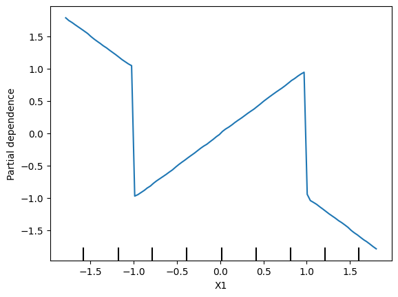
Correct
Uncomment the lines below for a hint or solution
取消以下几行注释以获得提示或解决方案
# q_6.hint()
q_6.solution()
Solution:
# There are many possible solutions.
# One example expression for y is.
y = -2 * X1 * (X1<-1) + X1 - 2 * X1 * (X1>1) - X2
# You don't need any more changes
Question 7
问题 7
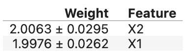
Create a dataset with 2 features and a target, such that the pdp of the first feature is flat, but its permutation importance is high. We will use a RandomForest for the model.
创建一个具有 2 个特征和一个目标的数据集,使得第一个特征的 pdp 是平坦的,但其排列重要性很高。我们将使用 RandomForest 作为模型。
Note: You only need to supply the lines that create the variables X1, X2 and y. The code to build the model and calculate insights is provided.
注意:您只需提供创建变量 X1、X2 和 y 的行。提供了构建模型和计算见解的代码。
import eli5
from eli5.sklearn import PermutationImportance

n_samples = 20000

# Create array holding predictive feature
# X1 = ____
# X2 = ____
X1 = 4 * rand(n_samples) - 2
X2 = 4 * rand(n_samples) - 2
# Create y. you should have X1 and X2 in the expression for y
# y = ____
y = X1 * X2

# create dataframe because pdp_isolate expects a dataFrame as an argument
my_df = pd.DataFrame({'X1': X1, 'X2': X2, 'y': y})
predictors_df = my_df.drop(['y'], axis=1)

my_model = RandomForestRegressor(n_estimators=30, random_state=1).fit(predictors_df, my_df.y)

disp = PartialDependenceDisplay.from_estimator(my_model, predictors_df, ['X1'], grid_resolution=300)
plt.show()

perm = PermutationImportance(my_model).fit(predictors_df, my_df.y)

# Check your answer
q_7.check()

# show the weights for the permutation importance you just calculated
eli5.show_weights(perm, feature_names = ['X1', 'X2'])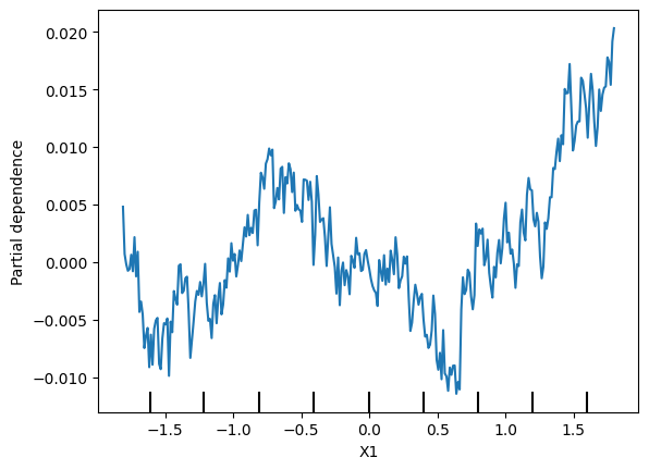
# Uncomment the following lines for the hint or solution
q_7.hint()
# q_7.solution()
Hint: You need for X1 to affect the prediction in order to have it affect permutation importance. But the average effect needs to be 0 to satisfy the PDP requirement. Achieve this by creating an interaction, so the effect of X1 depends on the value of X2 and vice-versa.
提示:您需要让 X1 影响预测,以便它影响排列重要性。但平均效应需要为 0 才能满足 PDP 要求。通过创建交互来实现这一点,因此 X1 的效果取决于 X2 的值,反之亦然。
Keep Going
继续
Partial dependence plots can be really interesting. We have a discussion thread to talk about what real-world topics or questions you'd be curious to see addressed with partial dependence plots.
部分依赖图真的很有趣。我们有一个讨论线程来讨论你想知道的部分依赖图如何解决现实世界中的主题或问题。
Next, learn how SHAP values help you understand the logic for each individual prediction.
接下来,了解SHAP 值如何帮助你理解每个预测的逻辑。