Welcome to Time Series!

欢迎来到时间序列！

Forecasting is perhaps the most common application of machine learning in the real world. Businesses forecast product demand, governments forecast economic and population growth, meteorologists forecast the weather. The understanding of things to come is a pressing need across science, government, and industry (not to mention our personal lives!), and practitioners in these fields are increasingly applying machine learning to address this need.

预测 可能是机器学习在现实世界中最常见的应用。企业预测产品需求，政府预测经济和人口增长，气象学家预测天气。了解未来是科学、政府和工业界（更不用说我们的个人生活了！）的迫切需求，这些领域的从业者越来越多地应用机器学习来满足这一需求。

Time series forecasting is a broad field with a long history. This course focuses on the application of modern machine learning methods to time series data with the goal of producing the most accurate predictions. The lessons in this course were inspired by winning solutions from past Kaggle forecasting competitions but will be applicable whenever accurate forecasts are a priority.

时间序列预测是一个历史悠久的广泛领域。本课程重点介绍将现代机器学习方法应用于时间序列数据，目的是产生最准确的预测。本课程中的课程灵感来自过去 Kaggle 预测竞赛的获奖解决方案，但只要准确预测是优先事项，它就会适用。

After finishing this course, you'll know how to:

完成本课程后，您将了解如何：

• engineer features to model the major time series components (trends, seasons, and cycles),
• 设计特征来模拟主要时间序列成分（趋势、季节和周期），
• visualize time series with many kinds of time series plots,
• 使用多种时间序列图可视化时间序列，
• create forecasting hybrids that combine the strengths of complementary models, and
• 创建结合互补模型优势的预测混合模型，以及
• adapt machine learning methods to a variety of forecasting tasks.
• 将机器学习方法应用于各种预测任务。

As part of the exercises, you'll get a chance to participate in our Store Sales - Time Series Forecasting Getting Started competition. In this competition, you're tasked with forecasting sales for Corporación Favorita (a large Ecuadorian-based grocery retailer) in almost 1800 product categories.

作为练习的一部分，您将有机会参加我们的 商店销售 - 时间序列预测 入门竞赛。在本次竞赛中，您的任务是预测 Corporación Favorita（一家大型厄瓜多尔杂货零售商）近 1800 个产品类别的销售额。

What is a Time Series?

什么是时间序列？

The basic object of forecasting is the time series, which is a set of observations recorded over time. In forecasting applications, the observations are typically recorded with a regular frequency, like daily or monthly.

预测的基本对象是时间序列，它是一组随时间记录的观察值。在预测应用中，观察结果通常以固定的频率记录，例如每日或每月。

import pandas as pd

df = pd.read_csv(
    "../input/ts-course-data/book_sales.csv",
    index_col='Date',
    parse_dates=['Date'],
).drop('Paperback', axis=1)

df.head()

	Hardcover
Date
2000-04-01	139
2000-04-02	128
2000-04-03	172
2000-04-04	139
2000-04-05	191

This series records the number of hardcover book sales at a retail store over 30 days. Notice that we have a single column of observations Hardcover with a time index Date.

本序列记录了零售店 30 天内精装书的销售数量。请注意，我们有一列观察值“精装书”，时间索引为“日期”。

Linear Regression with Time Series

时间序列线性回归

For the first part of this course, we'll use the linear regression algorithm to construct forecasting models. Linear regression is widely used in practice and adapts naturally to even complex forecasting tasks.

在本课程的第一部分，我们将使用线性回归算法构建预测模型。线性回归在实践中被广泛使用，甚至可以自然地适应复杂的预测任务。

The linear regression algorithm learns how to make a weighted sum from its input features. For two features, we would have:

线性回归算法学习如何从其输入特征中进行加权求和。对于两个特征，我们将有：

target = weight_1 * feature_1 + weight_2 * feature_2 + bias

During training, the regression algorithm learns values for the parameters weight_1, weight_2, and bias that best fit the target. (This algorithm is often called ordinary least squares since it chooses values that minimize the squared error between the target and the predictions.) The weights are also called regression coefficients and the bias is also called the intercept because it tells you where the graph of this function crosses the y-axis.

在训练期间，回归算法会学习最适合target的参数weight_1、weight_2和bias的值。 （该算法通常称为普通最小二乘法，因为它选择的值可最小化目标和预测之间的平方误差。）权重也称为回归系数，bias也称为截距，因为它告诉您此函数的图形与 y 轴的交点。

Time-step features

时间步长特征

There are two kinds of features unique to time series: time-step features and lag features.

时间序列有两种独有的特征：时间步长特征和滞后特征。

Time-step features are features we can derive directly from the time index. The most basic time-step feature is the time dummy, which counts off time steps in the series from beginning to end.

时间步长特征是我们可以直接从时间索引中得出的特征。最基本的时间步长特征是时间虚拟变量，它通过从序列的起点至终点按时间步长依次递增计数来表征时间推移。

import numpy as np

df['Time'] = np.arange(len(df.index))

df.head()

	Hardcover	Time
Date
2000-04-01	139	0
2000-04-02	128	1
2000-04-03	172	2
2000-04-04	139	3
2000-04-05	191	4

Linear regression with the time dummy produces the model:

使用时间虚拟变量进行线性回归可生成以下模型：

target = weight * time + bias

The time dummy then lets us fit curves to time series in a time plot, where Time forms the x-axis.

然后，时间虚拟变量让我们可以在时间图中将曲线拟合到时间序列中，其中Time构成 x 轴。

import matplotlib.pyplot as plt
import seaborn as sns
plt.style.use("seaborn-v0_8-whitegrid")
plt.rc(
    "figure",
    autolayout=True,
    figsize=(11, 4),
    titlesize=18,
    titleweight='bold',
)
plt.rc(
    "axes",
    labelweight="bold",
    labelsize="large",
    titleweight="bold",
    titlesize=16,
    titlepad=10,
)
%config InlineBackend.figure_format = 'retina'

fig, ax = plt.subplots()
ax.plot('Time', 'Hardcover', data=df, color='0.75')
ax = sns.regplot(x='Time', y='Hardcover', data=df, ci=None, scatter_kws=dict(color='0.25'))
ax.set_title('Time Plot of Hardcover Sales');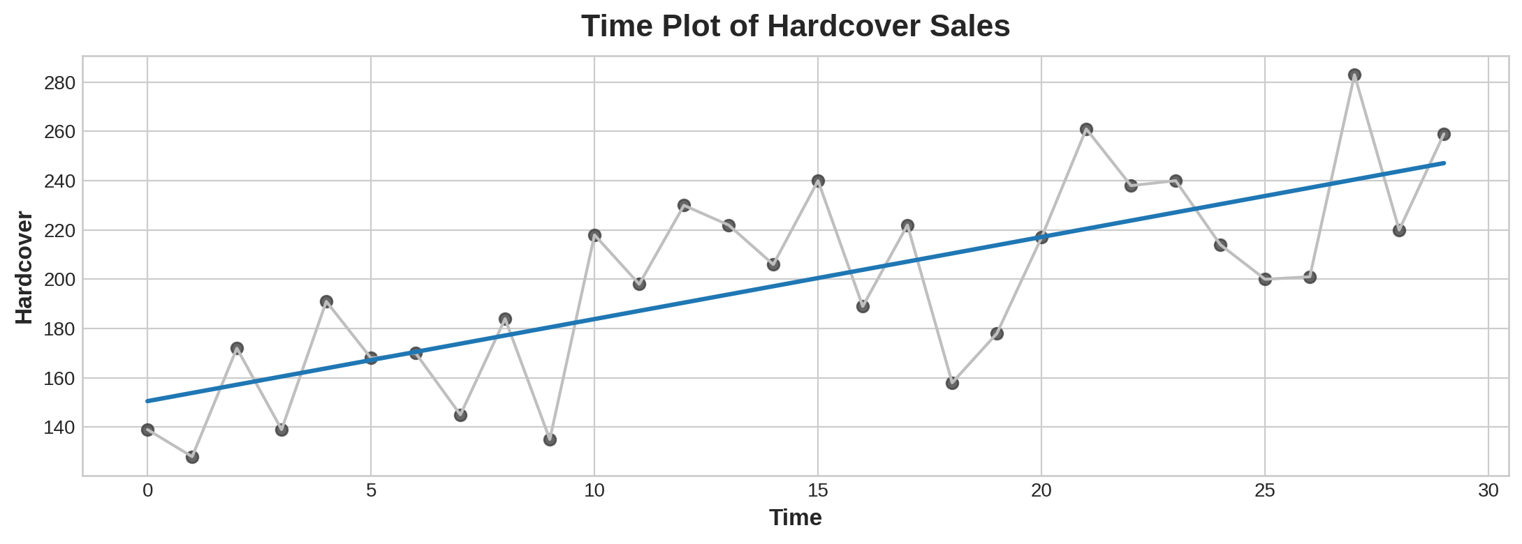

Time-step features let you model time dependence. A series is time dependent if its values can be predicted from the time they occured. In the Hardcover Sales series, we can predict that sales later in the month are generally higher than sales earlier in the month.

时间步长特征让您可以对时间依赖性进行建模。如果某个系列的值可以从其发生的时间进行预测，则该系列是时间依赖性的。在精装本销售系列中，我们可以预测当月晚些时候的销售额通常高于当月早些时候的销售额。

Lag features

滞后特征

To make a lag feature we shift the observations of the target series so that they appear to have occured later in time. Here we've created a 1-step lag feature, though shifting by multiple steps is possible too.

为了制作滞后特征，我们移动了目标系列的观察值，使它们看起来发生在较晚的时间。在这里，我们创建了一个 1 步滞后特征，尽管也可以移动多个步骤。

df['Lag_1'] = df['Hardcover'].shift(1)
df = df.reindex(columns=['Hardcover', 'Lag_1'])

df.head()

/usr/local/lib/python3.10/dist-packages/pandas/io/formats/format.py:1458: RuntimeWarning: invalid value encountered in greater
  has_large_values = (abs_vals > 1e6).any()
/usr/local/lib/python3.10/dist-packages/pandas/io/formats/format.py:1459: RuntimeWarning: invalid value encountered in less
  has_small_values = ((abs_vals < 10 ** (-self.digits)) & (abs_vals > 0)).any()
/usr/local/lib/python3.10/dist-packages/pandas/io/formats/format.py:1459: RuntimeWarning: invalid value encountered in greater
  has_small_values = ((abs_vals < 10 ** (-self.digits)) & (abs_vals > 0)).any()

	Hardcover	Lag_1
Date
2000-04-01	139	NaN
2000-04-02	128	139.0
2000-04-03	172	128.0
2000-04-04	139	172.0
2000-04-05	191	139.0

Linear regression with a lag feature produces the model:

具有滞后特征的线性回归产生模型：

target = weight * lag + bias

So lag features let us fit curves to lag plots where each observation in a series is plotted against the previous observation.

因此，滞后特征让我们能够将曲线拟合到滞后图，其中一系列中的每个观察值都与前一个观察值相对应。

fig, ax = plt.subplots()
ax = sns.regplot(x='Lag_1', y='Hardcover', data=df, ci=None, scatter_kws=dict(color='0.25'))
ax.set_aspect('equal')
ax.set_title('Lag Plot of Hardcover Sales');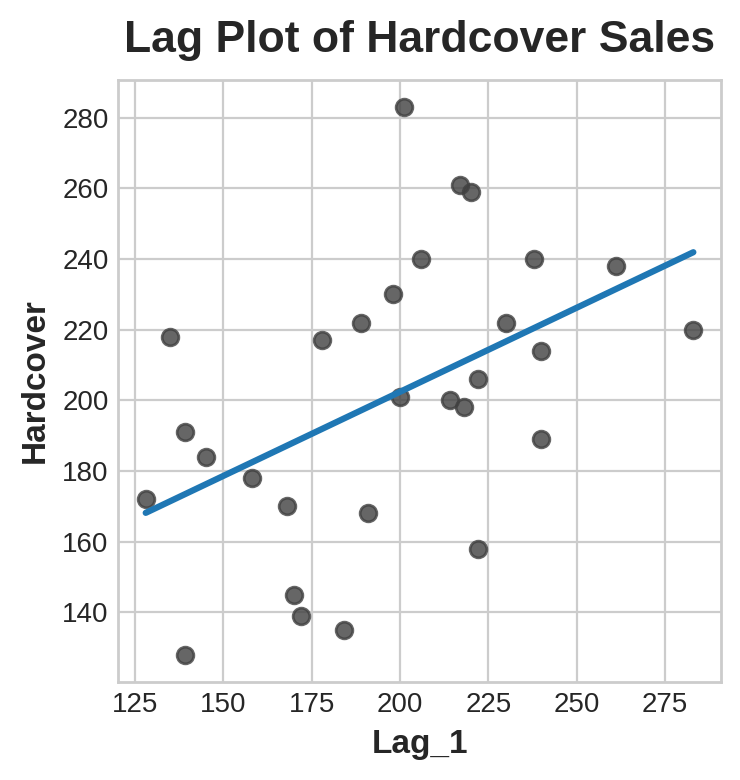

You can see from the lag plot that sales on one day (Hardcover) are correlated with sales from the previous day (Lag_1). When you see a relationship like this, you know a lag feature will be useful.

您可以从滞后图中看到，一天的销售额（精装本）与前一天的销售额（Lag_1）相关。当您看到这样的关系时，您就知道滞后特征会很有用。

More generally, lag features let you model serial dependence. A time series has serial dependence when an observation can be predicted from previous observations. In Hardcover Sales, we can predict that high sales on one day usually mean high sales the next day.

更一般地说，滞后特征可以让您对序列依赖性进行建模。当可以从先前的观察中预测观察结果时，时间序列具有序列依赖性。在精装本销售中，我们可以预测一天的高销售额通常意味着第二天的高销售额。

---

Adapting machine learning algorithms to time series problems is largely about feature engineering with the time index and lags. For most of the course, we use linear regression for its simplicity, but these features will be useful whichever algorithm you choose for your forecasting task.

将机器学习算法适应时间序列问题主要是关于使用时间索引和滞后进行特征工程。对于本课程的大部分内容，我们使用线性回归，因为它很简单，但无论您为预测任务选择哪种算法，这些功能都将很有用。

Example - Tunnel Traffic

示例 - 隧道交通

Tunnel Traffic is a time series describing the number of vehicles traveling through the Baregg Tunnel in Switzerland each day from November 2003 to November 2005. In this example, we'll get some practice applying linear regression to time-step features and lag features.

隧道交通 是一个时间序列，描述了 2003 年 11 月至 2005 年 11 月期间每天通过瑞士 Baregg 隧道的车辆数量。在此示例中，我们将练习将线性回归应用于时间步长特征和滞后特征。

The hidden cell sets everything up.

隐藏单元格设置了所有内容。

from pathlib import Path
from warnings import simplefilter

import matplotlib.pyplot as plt
import numpy as np
import pandas as pd

simplefilter("ignore")  # ignore warnings to clean up output cells

# Set Matplotlib defaults
plt.style.use("seaborn-whitegrid")
plt.rc("figure", autolayout=True, figsize=(11, 4))
plt.rc(
    "axes",
    labelweight="bold",
    labelsize="large",
    titleweight="bold",
    titlesize=14,
    titlepad=10,
)
plot_params = dict(
    color="0.75",
    style=".-",
    markeredgecolor="0.25",
    markerfacecolor="0.25",
    legend=False,
)
%config InlineBackend.figure_format = 'retina'

# Load Tunnel Traffic dataset
data_dir = Path("../input/ts-course-data")
tunnel = pd.read_csv(data_dir / "tunnel.csv", parse_dates=["Day"])

# Create a time series in Pandas by setting the index to a date
# column. We parsed "Day" as a date type by using `parse_dates` when
# loading the data.
tunnel = tunnel.set_index("Day")

# By default, Pandas creates a `DatetimeIndex` with dtype `Timestamp`
# (equivalent to `np.datetime64`, representing a time series as a
# sequence of measurements taken at single moments. A `PeriodIndex`,
# on the other hand, represents a time series as a sequence of
# quantities accumulated over periods of time. Periods are often
# easier to work with, so that's what we'll use in this course.
tunnel = tunnel.to_period()

tunnel.head()

	NumVehicles
Day
2003-11-01	103536
2003-11-02	92051
2003-11-03	100795
2003-11-04	102352
2003-11-05	106569

Time-step feature

时间步长特征

Provided the time series doesn't have any missing dates, we can create a time dummy by counting out the length of the series.

假设时间序列没有任何缺失日期，我们可以通过计算序列的长度来创建时间虚拟变量。

df = tunnel.copy()

df['Time'] = np.arange(len(tunnel.index))

df.head()

	NumVehicles	Time
Day
2003-11-01	103536	0
2003-11-02	92051	1
2003-11-03	100795	2
2003-11-04	102352	3
2003-11-05	106569	4

The procedure for fitting a linear regression model follows the standard steps for scikit-learn.

拟合线性回归模型的过程遵循 scikit-learn 的标准步骤。

from sklearn.linear_model import LinearRegression

# Training data
X = df.loc[:, ['Time']]  # features
y = df.loc[:, 'NumVehicles']  # target

# Train the model
model = LinearRegression()
model.fit(X, y)

# Store the fitted values as a time series with the same time index as
# the training data
y_pred = pd.Series(model.predict(X), index=X.index)

The model actually created is (approximately): Vehicles = 22.5 * Time + 98176. Plotting the fitted values over time shows us how fitting linear regression to the time dummy creates the trend line defined by this equation.

实际创建的模型为（大约）：车辆 = 22.5 * 时间 + 98176。绘制随时间变化的拟合值向我们展示了如何将线性回归拟合到时间虚拟变量中以创建由此方程定义的趋势线。

ax = y.plot(**plot_params)
ax = y_pred.plot(ax=ax, linewidth=3)
ax.set_title('Time Plot of Tunnel Traffic');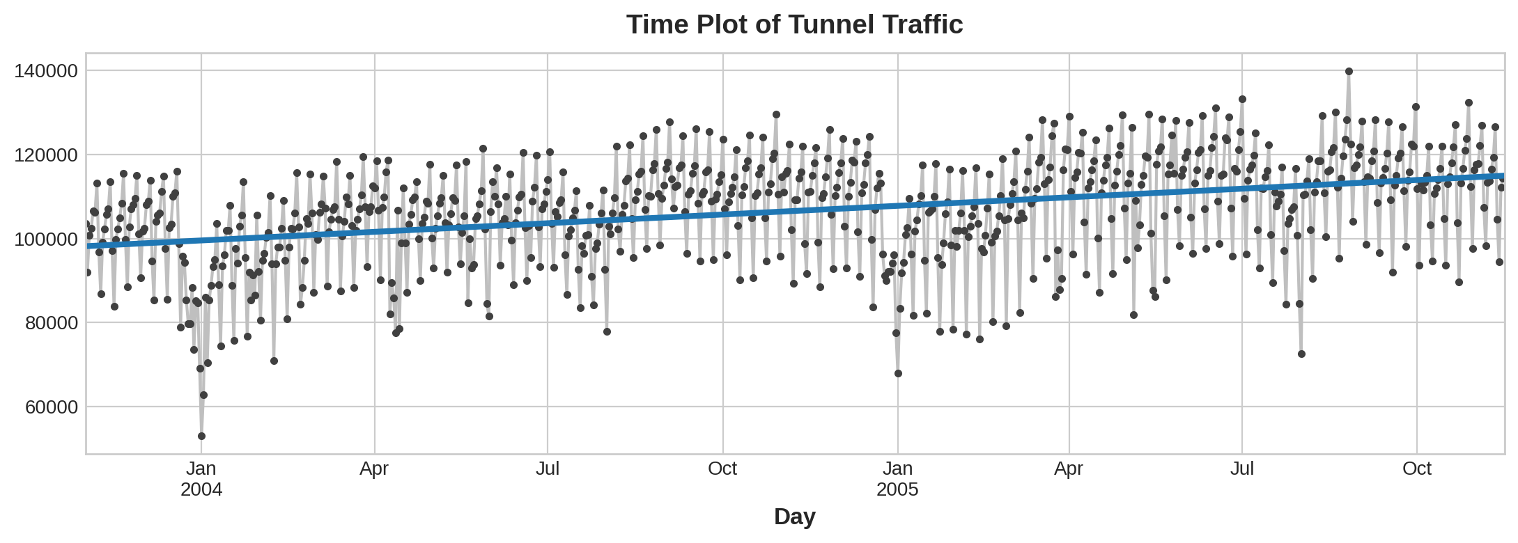

Lag feature

滞后特征

Pandas provides us a simple method to lag a series, the shift method.

Pandas 为我们提供了一种滞后序列的简单方法，即shift方法。

df['Lag_1'] = df['NumVehicles'].shift(1)
df.head()

	NumVehicles	Time	Lag_1
Day
2003-11-01	103536	0	NaN
2003-11-02	92051	1	103536.0
2003-11-03	100795	2	92051.0
2003-11-04	102352	3	100795.0
2003-11-05	106569	4	102352.0

When creating lag features, we need to decide what to do with the missing values produced. Filling them in is one option, maybe with 0.0 or "backfilling" with the first known value. Instead, we'll just drop the missing values, making sure to also drop values in the target from corresponding dates.

在创建滞后特征时，我们需要决定如何处理产生的缺失值。一种选择是将它们填充，可能是用 0.0 或用第一个已知值“向后填充”。相反，我们只需删除缺失值，确保也删除目标中相应日期的值。

from sklearn.linear_model import LinearRegression

X = df.loc[:, ['Lag_1']]
X.dropna(inplace=True)  # drop missing values in the feature set
y = df.loc[:, 'NumVehicles']  # create the target
y, X = y.align(X, join='inner')  # drop corresponding values in target

model = LinearRegression()
model.fit(X, y)

y_pred = pd.Series(model.predict(X), index=X.index)

The lag plot shows us how well we were able to fit the relationship between the number of vehicles one day and the number the previous day.

滞后图向我们展示了我们如何能够拟合一天的车辆数量和前一天车辆数量之间的关系。

fig, ax = plt.subplots()
ax.plot(X['Lag_1'], y, '.', color='0.25')
ax.plot(X['Lag_1'], y_pred)
ax.set_aspect('equal')
ax.set_ylabel('NumVehicles')
ax.set_xlabel('Lag_1')
ax.set_title('Lag Plot of Tunnel Traffic');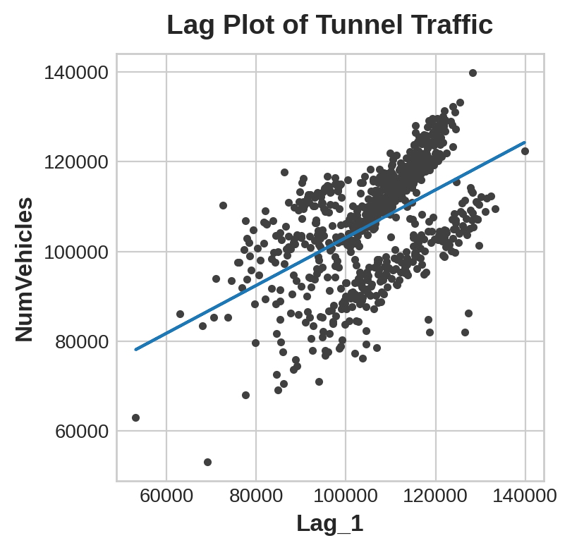

What does this prediction from a lag feature mean about how well we can predict the series across time? The following time plot shows us how our forecasts now respond to the behavior of the series in the recent past.

滞后特征的预测对我们能否跨时间预测序列意味着什么？以下时间图向我们展示了我们的预测现在如何响应近期序列的行为。

ax = y.plot(**plot_params)
ax = y_pred.plot()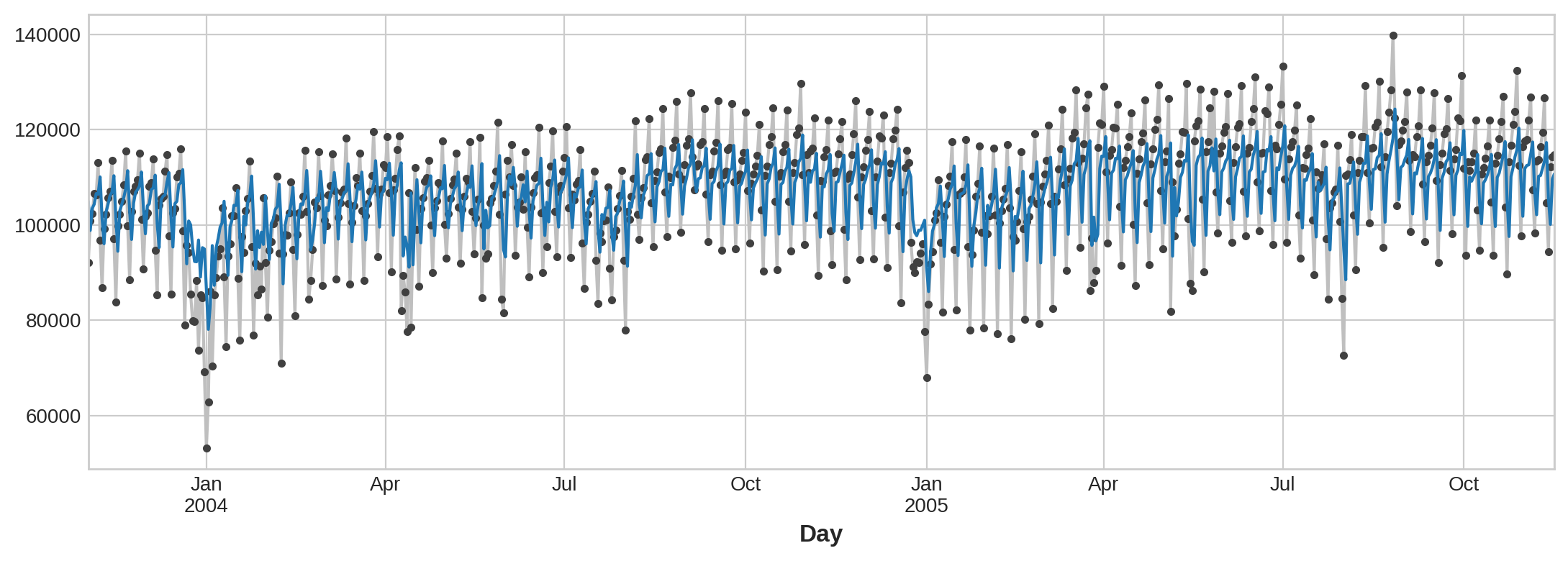

The best time series models will usually include some combination of time-step features and lag features. Over the next few lessons, we'll learn how to engineer features modeling the most common patterns in time series using the features from this lesson as a starting point.

最佳时间序列模型通常包括时间步长特征和滞后特征的某种组合。在接下来的几节课中，我们将学习如何使用本课中的特征作为起点来设计特征，以对时间序列中最常见的模式进行建模。

Your Turn

轮到你了

Move on to the Exercise, where you'll begin forecasting Store Sales using the techniques you learned in this tutorial.

继续练习，你将使用本教程中学到的技术开始 预测商店销售额。

---