This notebook is an exercise in the Time Series course. You can reference the tutorial at this link.

---

Introduction

简介

Run this cell to set everything up!

运行此单元完成所有设置！

# Setup feedback system
from learntools.core import binder
binder.bind(globals())
from learntools.time_series.ex1 import *

# Setup notebook
from pathlib import Path
from learntools.time_series.style import *  # plot style settings

import pandas as pd
import matplotlib.pyplot as plt
import numpy as np
import seaborn as sns
from sklearn.linear_model import LinearRegression

data_dir = Path('../input/ts-course-data/')
comp_dir = Path('../input/store-sales-time-series-forecasting')

book_sales = pd.read_csv(
    data_dir / 'book_sales.csv',
    index_col='Date',
    parse_dates=['Date'],
).drop('Paperback', axis=1)
book_sales['Time'] = np.arange(len(book_sales.index))
book_sales['Lag_1'] = book_sales['Hardcover'].shift(1)
book_sales = book_sales.reindex(columns=['Hardcover', 'Time', 'Lag_1'])

ar = pd.read_csv(data_dir / 'ar.csv')

dtype = {
    'store_nbr': 'category',
    'family': 'category',
    'sales': 'float32',
    'onpromotion': 'uint64',
}
store_sales = pd.read_csv(
    comp_dir / 'train.csv',
    dtype=dtype,
    parse_dates=['date'],
    # infer_datetime_format=True,
)
store_sales = store_sales.set_index('date').to_period('D')
store_sales = store_sales.set_index(['store_nbr', 'family'], append=True)
average_sales = store_sales.groupby('date').mean()['sales']

---

One advantage linear regression has over more complicated algorithms is that the models it creates are explainable -- it's easy to interpret what contribution each feature makes to the predictions. In the model target = weight * feature + bias, the weight tells you by how much the target changes on average for each unit of change in the feature.

线性回归相对于更复杂的算法的一个优势是，它创建的模型是可解释的——很容易解释每个特征对预测的贡献。在模型目标 = 权重 * 特征 + 偏差中，权重告诉你特征每个变化单位导致目标平均变化了多少。

Run the next cell to see a linear regression on Hardcover Sales.

运行下一个单元格，查看精装本销量的线性回归。

fig, ax = plt.subplots()
ax.plot('Time', 'Hardcover', data=book_sales, color='0.75')
ax = sns.regplot(x='Time', y='Hardcover', data=book_sales, ci=None, scatter_kws=dict(color='0.25'))
ax.set_title('Time Plot of Hardcover Sales');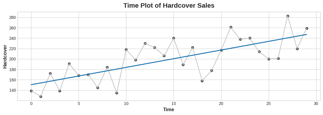

1) Interpret linear regression with the time dummy

1) 用时间虚拟变量解释线性回归

The linear regression line has an equation of (approximately) Hardcover = 3.33 * Time + 150.5. Over 6 days how much on average would you expect hardcover sales to change? After you've thought about it, run the next cell.

线性回归线的方程式约为精装书 = 3.33 * 时间 + 150.5。你预计6天内精装书的销量平均会变化多少？思考完毕后，运行下一个单元。

# View the solution (Run this line to receive credit!)
# 6*3.33 = 20
q_1.check()

Correct:

A change of 6 steps in Time corresponds to an average change of 6 * 3.33 = 19.98 in Hardcover sales.

时间变化 6 天对应精装书销量平均变化 6 * 3.33 = 19.98。

# Uncomment the next line for a hint
q_1.hint()

Hint: Do you remember the slope-intercept equation of a line? The slope is 3.33, so Hardcover will change on average by 3.33 units for every 1 step change in Time, according to this model.

提示：你还记得直线的斜率截距方程吗？斜率为 3.33，因此根据该模型，时间每变化一步，精装书销量 的平均变化量就会为 3.33 个单位。

---

Interpreting the regression coefficients can help us recognize serial dependence in a time plot. Consider the model target = weight * lag_1 + error, where error is random noise and weight is a number between -1 and 1. The weight in this case tells you how likely the next time step will have the same sign as the previous time step: a weight close to 1 means target will likely have the same sign as the previous step, while a weight close to -1 means target will likely have the opposite sign.

解读回归系数有助于我们识别时间图中的序列依赖性。考虑模型目标 = 权重 * 滞后 1 + 误差，其中误差是随机噪声，权重是介于 -1 和 1 之间的数字。在这种情况下，权重表示下一个时间步与上一个时间步具有相同符号的可能性：接近 1 的权重表示目标可能与上一个时间步具有相同符号，而接近 -1 的权重表示目标可能具有相反的符号。

2) Interpret linear regression with a lag feature

2) 解读具有滞后特征的线性回归

Run the following cell to see two series generated according to the model just described.

运行以下单元格，查看根据上述模型生成的两个序列。

fig, (ax1, ax2) = plt.subplots(2, 1, figsize=(11, 5.5), sharex=True)
ax1.plot(ar['ar1'])
ax1.set_title('Series 1')
ax2.plot(ar['ar2'])
ax2.set_title('Series 2');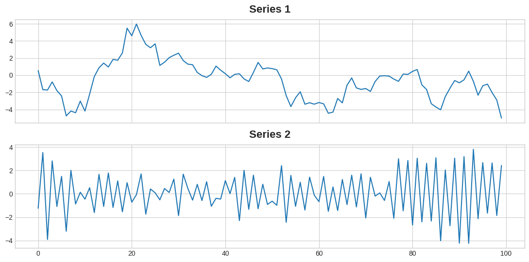

One of these series has the equation target = 0.95 * lag_1 + error and the other has the equation target = -0.95 * lag_1 + error, differing only by the sign on the lag feature. Can you tell which equation goes with each series?

其中一个序列的方程式为目标 = 0.95 * 滞后 1 + 误差，另一个序列的方程式为目标 = -0.95 * 滞后 1 + 误差，两者仅在滞后特征的符号上有所不同。你能分辨出每个序列对应的方程式吗？

# View the solution (Run this cell to receive credit!)
# Series1 0.95 & Series -0.95
q_2.check()

Correct:

Series 1 was generated by target = 0.95 * lag_1 + error and Series 2 was generated by target = -0.95 * lag_1 + error.

Series 1 由target = 0.95 * lag_1 + error生成，Series 2 由target = -0.95 * lag_1 + error生成。

# Uncomment the next line for a hint
q_2.hint()

Hint: The series with the 0.95 weight will tend to have values with signs that stay the same. The series with the -0.95 weight will tend to have values with signs that change back and forth.

提示：权重为 0.95 的序列，其值的符号趋于保持不变。权重为 -0.95 的序列，其值的符号趋于来回变化。

---

Now we'll get started with the Store Sales - Time Series Forecasting competition data. The entire dataset comprises almost 1800 series recording store sales across a variety of product families from 2013 into 2017. For this lesson, we'll just work with a single series (average_sales) of the average sales each day.

现在我们将开始使用 商店销售额 - 时间序列预测 竞赛数据。整个数据集包含近 1800 个系列，记录了 2013 年至 2017 年期间各种产品系列的商店销售额。在本课中，我们将只使用一个包含每日平均销售额的系列（average_sales）。

3) Fit a time-step feature

3) 拟合时间步长特征

Complete the code below to create a linear regression model with a time-step feature on the series of average product sales. The target is in a column called 'sales'.

完成以下代码，创建一个基于平均产品销售额系列的具有时间步长特征的线性回归模型。目标位于名为sales的列中。

from sklearn.linear_model import LinearRegression

df = average_sales.to_frame()

# YOUR CODE HERE: Create a time dummy
# time = ____
time = np.arange(len(df.index))

df['time'] = time 

# YOUR CODE HERE: Create training data
# X = ____  # features
# y = ____  # target
X = df[['time']]
y = df['sales']

# Train the model
model = LinearRegression()
model.fit(X, y)

# Store the fitted values as a time series with the same time index as
# the training data
y_pred = pd.Series(model.predict(X), index=X.index)

# Check your answer
q_3.check()

Correct

# Lines below will give you a hint or solution code
# q_3.hint()
# q_3.solution()

Run this cell if you'd like to see a plot of the result.

如果您想查看结果图，请运行此单元格。

ax = y.plot(**plot_params, alpha=0.5)
ax = y_pred.plot(ax=ax, linewidth=3)
ax.set_title('Time Plot of Total Store Sales');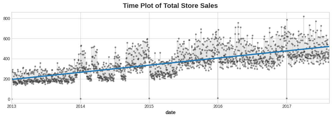

---

4) Fit a lag feature to Store Sales

4) 为商店销售额拟合滞后特征

Complete the code below to create a linear regression model with a lag feature on the series of average product sales. The target is in a column of df called 'sales'.

完成以下代码，创建一个基于平均产品销售额序列的具有滞后特征的线性回归模型。目标值位于df中名为'sales'的列中。

df = average_sales.to_frame()

# YOUR CODE HERE: Create a lag feature from the target 'sales'
# lag_1 = ____
lag_1 = df['sales'].shift(1)

df['lag_1'] = lag_1  # add to dataframe

X = df.loc[:, ['lag_1']].dropna()  # features
y = df.loc[:, 'sales']  # target
y, X = y.align(X, join='inner')  # drop corresponding values in target

# YOUR CODE HERE: Create a LinearRegression instance and fit it to X and y.
# model = ____

model = LinearRegression()
model.fit(X, y)

# YOUR CODE HERE: Create Store the fitted values as a time series with
# the same time index as the training data
# y_pred = ____
y_pred = pd.Series(model.predict(X), index=X.index)

# Check your answer
q_4.check()

Correct

# Lines below will give you a hint or solution code
# q_4.hint()
# q_4.solution()

Run the next cell if you'd like to see the result.

如果您想查看结果，请运行下一个单元格。

fig, ax = plt.subplots()
ax.plot(X['lag_1'], y, '.', color='0.25')
ax.plot(X['lag_1'], y_pred)
ax.set(aspect='equal', ylabel='sales', xlabel='lag_1', title='Lag Plot of Average Sales');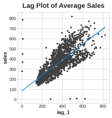

Keep Going

继续

Model trend in time series with moving average plots and the time dummy.

趋势模型 使用移动平均图和时间虚拟变量构建时间序列趋势模型。

---