What is Trend?
什么是趋势?
The trend component of a time series represents a persistent, long-term change in the mean of the series. The trend is the slowest-moving part of a series, the part representing the largest time scale of importance. In a time series of product sales, an increasing trend might be the effect of a market expansion as more people become aware of the product year by year.
时间序列的趋势部分表示序列平均值的持续、长期变化。趋势是序列中变化最慢的部分,代表着最重要的时间尺度。在产品销售的时间序列中,上升趋势可能是市场扩张的结果,因为越来越多的人逐年了解该产品。
In this course, we'll focus on trends in the mean. More generally though, any persistent and slow-moving change in a series could constitute a trend -- time series commonly have trends in their variation for instance.
在本课程中,我们将重点关注平均值的趋势。更一般地说,序列中任何持续且缓慢的变化都可能构成趋势——例如,时间序列的变化通常具有趋势。
Moving Average Plots
移动平均图
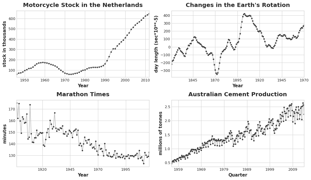
To see what kind of trend a time series might have, we can use a moving average plot. To compute a moving average of a time series, we compute the average of the values within a sliding window of some defined width. Each point on the graph represents the average of all the values in the series that fall within the window on either side. The idea is to smooth out any short-term fluctuations in the series so that only long-term changes remain.
为了了解时间序列可能具有的趋势类型,我们可以使用移动平均图。要计算时间序列的移动平均数,我们计算某个定义宽度的滑动窗口内值的平均值。图上的每个点代表序列中位于窗口两侧的所有值的平均值。这样做的目的是平滑序列中的任何短期波动,以便只保留长期变化。
Notice how the Mauna Loa series above has a repeating up and down movement year after year -- a short-term, seasonal change. For a change to be a part of the trend, it should occur over a longer period than any seasonal changes. To visualize a trend, therefore, we take an average over a period longer than any seasonal period in the series. For the Mauna Loa series, we chose a window of size 12 to smooth over the season within each year.
请注意,上图的 莫纳罗亚火山 序列年复一年地重复着上下波动——这是一种短期的 季节性 变化。要使变化成为趋势的一部分,它发生的周期应该比任何季节性变化都要长。因此,为了直观地呈现趋势,我们取比序列中任何季节性周期都长的周期的平均值。对于 莫纳罗亚火山 序列,我们选择了大小为 12 的窗口来平滑每年的季节变化。
Engineering Trend
趋势的工程化
Once we've identified the shape of the trend, we can attempt to model it using a time-step feature. We've already seen how using the time dummy itself will model a linear trend:
一旦我们确定了趋势的形状,就可以尝试使用时间步长特征对其进行建模。我们已经了解了如何使用时间虚拟变量本身来建模线性趋势:
target = a * time + bWe can fit many other kinds of trend through transformations of the time dummy. If the trend appears to be quadratic (a parabola), we just need to add the square of the time dummy to the feature set, giving us:
我们可以通过时间虚拟变量的变换来拟合许多其他类型的趋势。如果趋势呈现二次函数(抛物线),我们只需将时间虚拟变量的平方添加到特征集中,即可得到:
target = a * time ** 2 + b * time + cLinear regression will learn the coefficients a, b, and c.
线性回归将拟合系数a、b和c。
The trend curves in the figure below were both fit using these kinds of features and scikit-learn's LinearRegression:
下图中的趋势曲线均使用这类特征和 scikit-learn 的线性回归进行拟合:
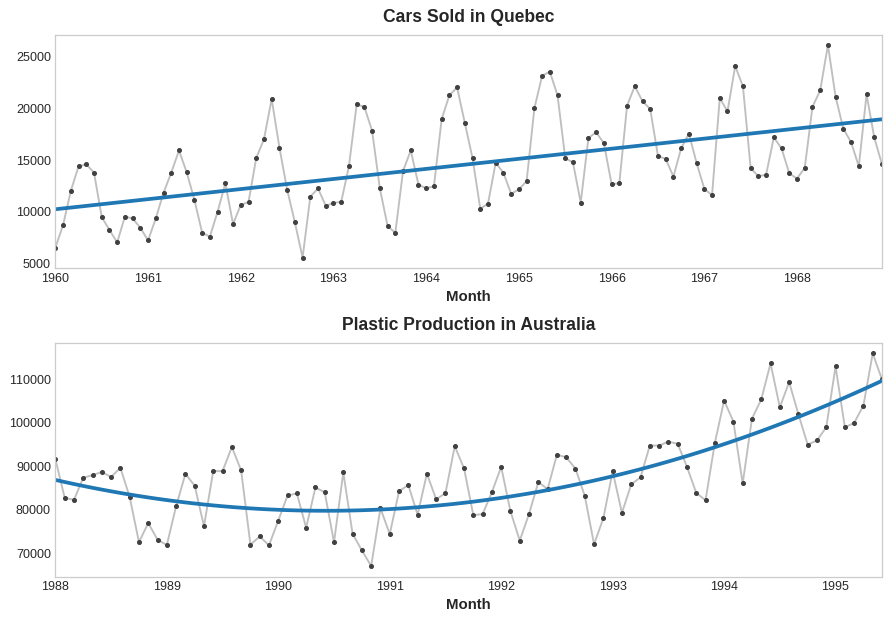
If you haven't seen the trick before, you may not have realized that linear regression can fit curves other than lines. The idea is that if you can provide curves of the appropriate shape as features, then linear regression can learn how to combine them in the way that best fits the target.
如果您之前没见过这个技巧,您可能没有意识到线性回归可以拟合曲线而不是直线。其原理是,如果您能提供适当形状的曲线作为特征,那么线性回归就能学习如何以最符合目标的方式组合它们。
Example - Tunnel Traffic
示例 - 隧道流量
In this example we'll create a trend model for the Tunnel Traffic dataset.
在本例中,我们将为 隧道流量 数据集创建一个趋势模型。
from pathlib import Path
from warnings import simplefilter
import matplotlib.pyplot as plt
import numpy as np
import pandas as pd
simplefilter("ignore") # ignore warnings to clean up output cells
# Set Matplotlib defaults
plt.style.use("seaborn-whitegrid")
plt.rc("figure", autolayout=True, figsize=(11, 5))
plt.rc(
"axes",
labelweight="bold",
labelsize="large",
titleweight="bold",
titlesize=14,
titlepad=10,
)
plot_params = dict(
color="0.75",
style=".-",
markeredgecolor="0.25",
markerfacecolor="0.25",
legend=False,
)
%config InlineBackend.figure_format = 'retina'
# Load Tunnel Traffic dataset
data_dir = Path("../input/ts-course-data")
tunnel = pd.read_csv(data_dir / "tunnel.csv", parse_dates=["Day"])
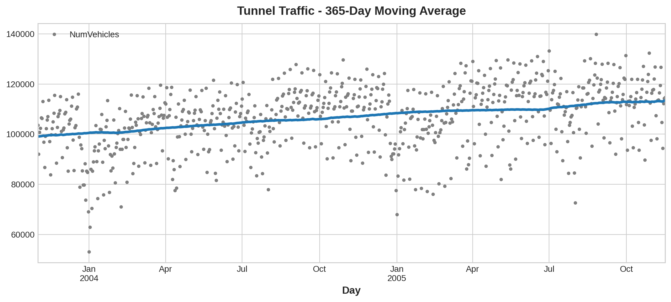
tunnel = tunnel.set_index("Day").to_period()Let's make a moving average plot to see what kind of trend this series has. Since this series has daily observations, let's choose a window of 365 days to smooth over any short-term changes within the year.
让我们绘制一个移动平均线图来观察这个序列的趋势。由于这个序列包含每日观测值,因此我们选择一个 365 天的窗口来平滑一年内的任何短期变化。
To create a moving average, first use the rolling method to begin a windowed computation. Follow this by the mean method to compute the average over the window. As we can see, the trend of Tunnel Traffic appears to be about linear.
要创建移动平均线,首先使用滚动方法开始窗口计算。然后使用平均值方法计算窗口平均值。如我们所见,隧道流量 的趋势似乎呈线性。
moving_average = tunnel.rolling(
    window=365,       # 365-day window
    center=True,      # puts the average at the center of the window
    min_periods=183,  # choose about half the window size
).mean()              # compute the mean (could also do median, std, min, max, ...)

ax = tunnel.plot(style=".", color="0.5")
moving_average.plot(
    ax=ax, linewidth=3, title="Tunnel Traffic - 365-Day Moving Average", legend=False,
);
In Lesson 1, we engineered our time dummy in Pandas directly. From now on, however, we'll use a function from the statsmodels library called DeterministicProcess. Using this function will help us avoid some tricky failure cases that can arise with time series and linear regression. The order argument refers to polynomial order: 1 for linear, 2 for quadratic, 3 for cubic, and so on.
在第一课中,我们直接在 Pandas 中构建了时间虚拟变量。不过,从现在开始,我们将使用 statsmodels 库中一个名为 DeterministicProcess 的函数。使用此函数可以帮助我们避免时间序列和线性回归中可能出现的一些棘手的失败情况。order 参数指的是多项式的阶数:1 表示一次,2 表示二次,3 表示三次,依此类推。
from statsmodels.tsa.deterministic import DeterministicProcess

dp = DeterministicProcess(
    index=tunnel.index,  # dates from the training data
    constant=True,       # dummy feature for the bias (y_intercept)
    order=1,             # the time dummy (trend)
    drop=True,           # drop terms if necessary to avoid collinearity
)
# `in_sample` creates features for the dates given in the `index` argument
X = dp.in_sample()

X.head()| const | trend | |
|---|---|---|
| Day | ||
| 2003-11-01 | 1.0 | 1.0 |
| 2003-11-02 | 1.0 | 2.0 |
| 2003-11-03 | 1.0 | 3.0 |
| 2003-11-04 | 1.0 | 4.0 |
| 2003-11-05 | 1.0 | 5.0 |
(A deterministic process, by the way, is a technical term for a time series that is non-random or completely determined, like the const and trend series are. Features derived from the time index will generally be deterministic.)
(顺便说一下, 确定性过程 是一个技术术语,指的是非随机或完全 确定 的时间序列,例如 const 和 trend 序列。从时间索引得出的特征通常是确定性的。)
We create our trend model basically as before, though note the addition of the fit_intercept=False argument.
我们像以前一样创建基础趋势模型,但请注意添加了 fit_intercept=False 参数。
from sklearn.linear_model import LinearRegression

y = tunnel["NumVehicles"]  # the target

# The intercept is the same as the `const` feature from
# DeterministicProcess. LinearRegression behaves badly with duplicated
# features, so we need to be sure to exclude it here.

# 截距与 DeterministicProcess 中的 `const` 特征相同。
# 线性回归在处理重复特征时表现不佳,因此我们需要确保在此处将其排除。

model = LinearRegression(fit_intercept=False)
model.fit(X, y)

y_pred = pd.Series(model.predict(X), index=X.index)
The trend discovered by our LinearRegression model is almost identical to the moving average plot, which suggests that a linear trend was the right decision in this case.
我们的线性回归模型发现的趋势与移动平均图几乎相同,这表明在这种情况下线性趋势是正确的决定。
ax = tunnel.plot(style=".", color="0.5", title="Tunnel Traffic - Linear Trend")
_ = y_pred.plot(ax=ax, linewidth=3, label="Trend")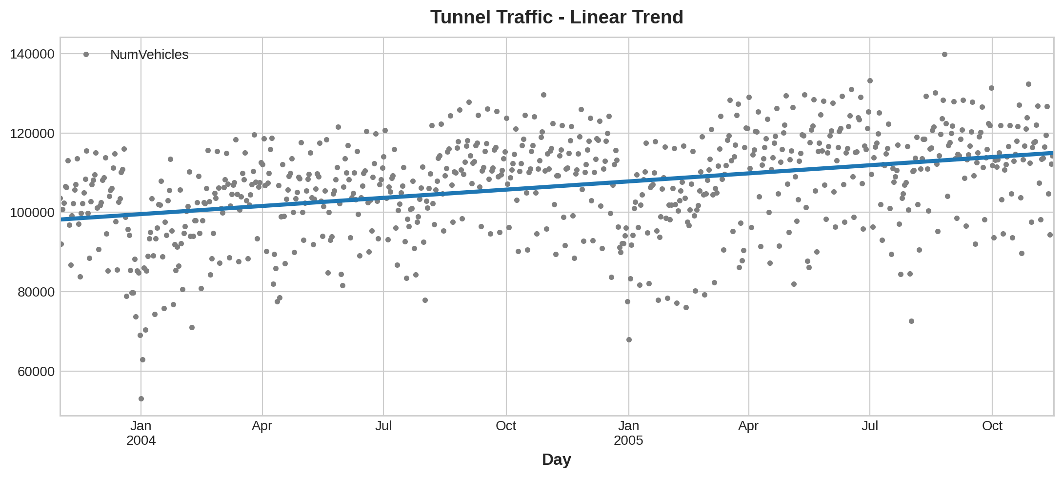
To make a forecast, we apply our model to "out of sample" features. "Out of sample" refers to times outside of the observation period of the training data. Here's how we could make a 30-day forecast:
为了进行预测,我们将模型应用于样本外特征。样本外是指训练数据观察期之外的时间。以下是进行 30 天预测的方法:
X = dp.out_of_sample(steps=30)

y_fore = pd.Series(model.predict(X), index=X.index)

y_fore.head()
2005-11-17 114981.801146
2005-11-18 115004.298595
2005-11-19 115026.796045
2005-11-20 115049.293494
2005-11-21 115071.790944
Freq: D, dtype: float64Let's plot a portion of the series to see the trend forecast for the next 30 days:
让我们绘制该系列的一部分来查看未来 30 天的趋势预测:
ax = tunnel["2005-05":].plot(title="Tunnel Traffic - Linear Trend Forecast", **plot_params)
ax = y_pred["2005-05":].plot(ax=ax, linewidth=3, label="Trend")
ax = y_fore.plot(ax=ax, linewidth=3, label="Trend Forecast", color="C3")
_ = ax.legend()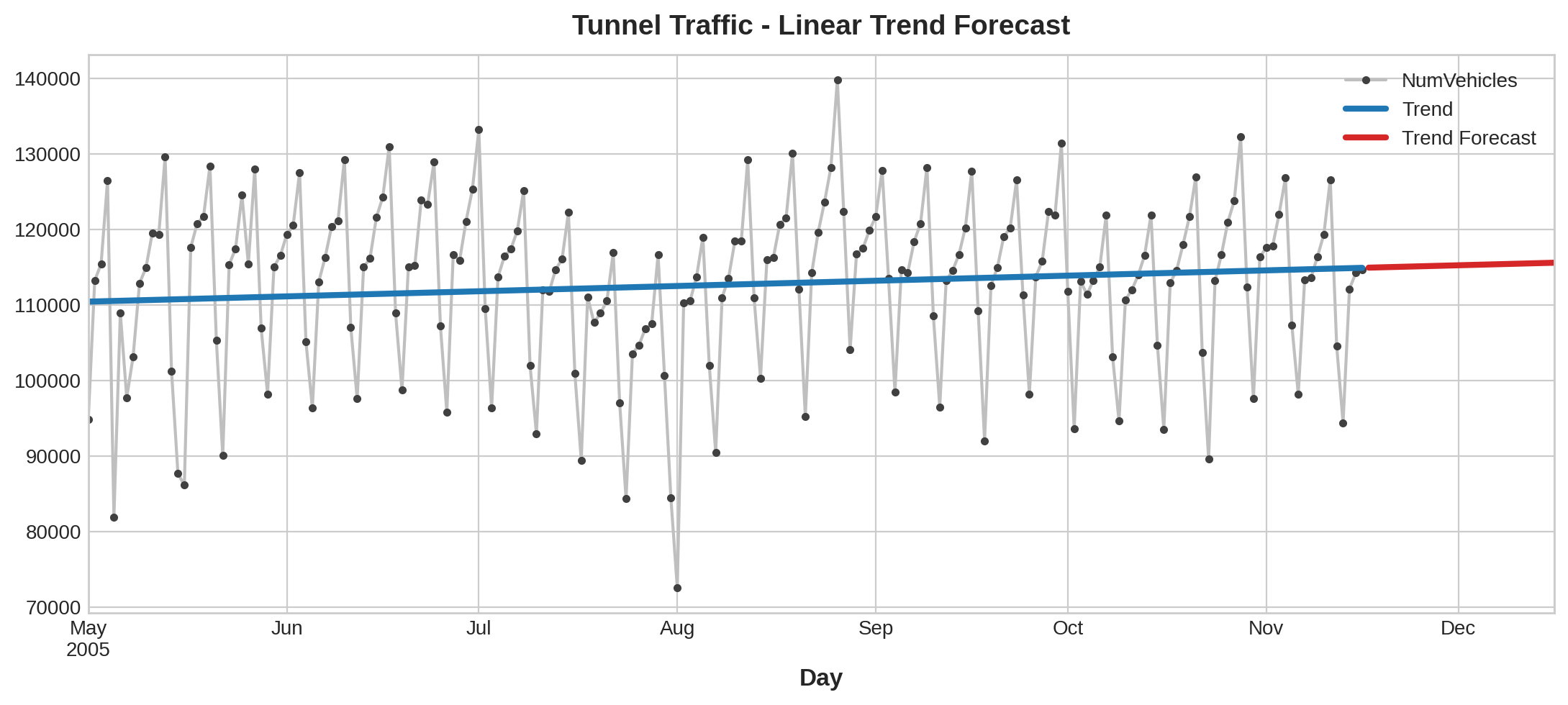
The trend models we learned about in this lesson turn out to be useful for a number of reasons. Besides acting as a baseline or starting point for more sophisticated models, we can also use them as a component in a "hybrid model" with algorithms unable to learn trends (like XGBoost and random forests). We'll learn more about this technique in Lesson 5.
我们在本课中学习的趋势模型被证明非常有用,原因有很多。除了作为更复杂模型的基线或起点之外,我们还可以将它们用作“混合模型”的组成部分,用于那些无法学习趋势的算法(例如 XGBoost 和随机森林)。我们将在第五课中详细了解这项技术。
Your Turn
轮到你了
Model trend in Store Sales and understand the risks of forecasting with high-order polynomials.
商店销售趋势模型 并了解使用高阶多项式进行预测的风险。
Have questions or comments? Visit the course discussion forum to chat with other learners.