Welcome to Data Visualization!

欢迎来到数据可视化！

In this hands-on course, you'll learn how to take your data visualizations to the next level with seaborn, a powerful but easy-to-use data visualization tool. To use seaborn, you'll also learn a bit about how to write code in Python, a popular programming language. That said,

在本实践课程中，您将学习如何使用 seaborn 将数据可视化提升到一个新的水平，这是一个功能强大但易于使用的数据 可视化工具。 要使用seaborn，您还将了解如何使用流行的编程语言Python 编写代码。 也就是说，

• the course is aimed at those with no prior programming experience, and
• 该课程针对那些没有编程经验的人，并且
• each chart uses short and simple code, making seaborn much faster and easier to use than many other data visualization tools (such as Excel, for instance).
• 每个图表都使用简短的代码，使seaborn比许多其他数据可视化工具（例如Excel）更快更容易使用。

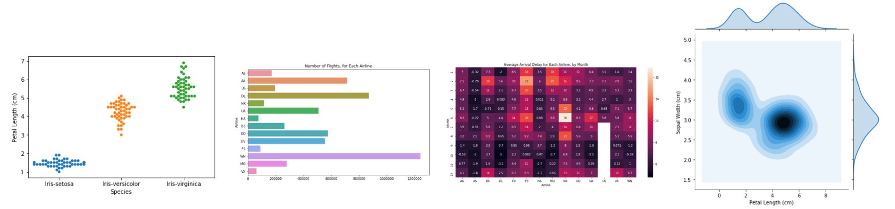
So, if you've never written a line of code, and you want to learn the bare minimum to start making faster, more attractive plots today, you're in the right place! To take a peek at some of the charts you'll make, check out the figures below.

因此，如果您从未编写过一行代码，并且想要学习 最低限度 的知识来开始制作更快、更有吸引力的绘图，那么您来对地方了！ 要查看您将制作的一些图表，请查看下图。

Your coding environment

你的编码环境

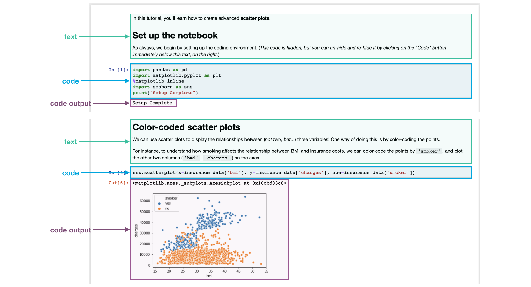
Take the time now to scroll quickly up and down this page. You'll notice that there are a lot of different types of information, including:

现在花点时间快速上下滚动此页面。 您会注意到有很多不同类型的信息，包括：

1. text (like the text you're reading right now!),
2. 文本（就像您现在正在阅读的文本！），
3. code (which is always contained inside a gray box called a code cell), and
4. 代码（始终包含在称为代码单元的灰色框中），以及
5. code output (or the printed result from running code that always appears immediately below the corresponding code).
6. 代码输出（或运行代码的打印结果，始终出现在相应代码的正下方）。

We refer to these pages as Jupyter notebooks (or, often just notebooks), and we'll work with them throughout the mini-course. Another example of a notebook can be found in the image below.

我们将这些页面称为 Jupyter 笔记本（或者，通常只是 笔记本），我们将在整个迷你课程中使用它们。 下图中可以找到笔记本的另一个示例。

In the notebook you're reading now, we've already run all of the code for you. Soon, you will work with a notebook that allows you to write and run your own code!

在您现在正在阅读的笔记本中，我们已经为您运行了所有代码。 很快，您将使用一个笔记本来编写和运行自己的代码！

Set up the notebook

设置笔记本

There are a few lines of code that you'll need to run at the top of every notebook to set up your coding environment. It's not important to understand these lines of code now, and so we won't go into the details just yet. (_Notice that it returns as output: MARKDOWN_HASHaf83f68ce7454a908814a2ec40175297MARKDOWNHASH.)

您需要在每个笔记本的顶部运行几行代码来设置编码环境。 现在理解这些代码行并不重要，因此我们暂时不讨论细节。 （_注意它返回为输出：MARKDOWN_HASHaf83f68ce7454a908814a2ec40175297MARKDOWNHASH.）

import pandas as pd
pd.plotting.register_matplotlib_converters()
import matplotlib.pyplot as plt
%matplotlib inline
import seaborn as sns
print("Setup Complete")

Setup Complete

Load the data

加载数据

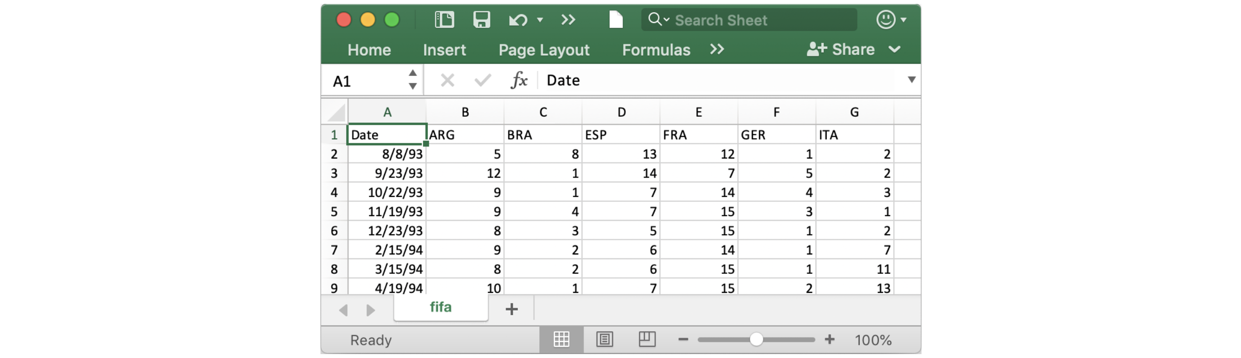
In this notebook, we'll work with a dataset of historical FIFA rankings for six countries: Argentina (ARG), Brazil (BRA), Spain (ESP), France (FRA), Germany (GER), and Italy (ITA). The dataset is stored as a CSV file (short for comma-separated values file). Opening the CSV file in Excel shows a row for each date, along with a column for each country.

在此笔记本中，我们将使用六个国家/地区的历史 FIFA 排名数据集：阿根廷 (ARG)、巴西 (BRA)、西班牙 (ESP)、法国 (FRA)、德国 (GER) 和意大利 (ITA)。 数据集存储为 CSV 文件(逗号分隔值文件) 的缩写）。在 Excel 中打开 CSV 文件会显示每个日期的一行以及每个国家/地区的一列 。

To load the data into the notebook, we'll use two distinct steps, implemented in the code cell below as follows:

要将数据加载到笔记本中，我们将使用两个不同的步骤，在下面的代码单元中实现，如下所示：

• begin by specifying the location (or filepath) where the dataset can be accessed, and then
• 首先指定可以访问数据集的位置（或文件路径），然后
• use the filepath to load the contents of the dataset into the notebook.
• 使用文件路径将数据集的内容加载到笔记本中。

# Path of the file to read
fifa_filepath = "../00 datasets/alexisbcook/data-for-datavis/fifa.csv"

# Read the file into a variable fifa_data
fifa_data = pd.read_csv(fifa_filepath, index_col="Date", parse_dates=True)

Note that the code cell above has four different lines.

请注意，上面的代码单元有 四 条不同的行。

Comments

注释

Two of the lines are preceded by a pound sign (#) and contain text that appears faded and italicized.

其中两行前面有井号 ( # )，并且包含淡化和斜体的文本。

Both of these lines are completely ignored by the computer when the code is run, and they only appear here so that any human who reads the code can quickly understand it. We refer to these two lines as comments, and it's good practice to include them to make sure that your code is readily interpretable.

当代码运行时，这两行代码都被计算机完全忽略，它们只出现在这里，以便任何阅读代码的人都可以快速理解它。 我们将这两行称为注释，最好的做法是包含它们以确保您的代码易于解释。

Executable code

可执行代码

The other two lines are executable code, or code that is run by the computer (in this case, to find and load the dataset).

另外两行是可执行代码，或由计算机运行的代码（在本例中，用于查找并加载数据集）。

The first line sets the value of fifa_filepath to the location where the dataset can be accessed. In this case, we've provided the filepath for you (in quotation marks). Note that the comment immediately above this line of executable code provides a quick description of what it does!

第一行将fifa_filepath的值设置为可以访问数据集的位置。 在本例中，我们已为您提供了文件路径（用引号引起来）。 请注意，此行可执行代码上方的注释提供了其功能的快速描述！

The second line sets the value of fifa_data to contain all of the information in the dataset. This is done with pd.read_csv. It is immediately followed by three different pieces of text (underlined in the image above) that are enclosed in parentheses and separated by commas. These are used to customize the behavior when the dataset is loaded into the notebook:

第二行设置fifa_data的值以包含数据集中的所有信息。 这是通过pd.read_csv完成的。 紧随其后的是三个不同的文本片段（上图中带下划线的文本），它们括在括号中并用逗号分隔。 这些用于自定义将数据集加载到笔记本中时的行为：

• fifa_filepath - The filepath for the dataset always needs to be provided first.
• fifa_filepath - 始终需要首先提供数据集的文件路径。
• index_col="Date" - When we load the dataset, we want each entry in the first column to denote a different row. To do this, we set the value of index_col to the name of the first column ("Date", found in cell A1 of the file when it's opened in Excel).
• index_col="Date" - 当我们加载数据集时，我们希望第一列中的每个条目表示不同的行。 为此，我们将index_col的值设置为第一列的名称（Date，在 Excel 中打开文件时可在文件的单元格 A1 中找到）。
• parse_dates=True - This tells the notebook to understand the each row label as a date (as opposed to a number or other text with a different meaning).
• parse_dates=True - 这告诉笔记本将每行的标签理解为日期（而不是数字或其他具有不同含义的文本）。

These details will make more sense soon, when you have a chance to load your own dataset in a hands-on exercise.

当您有机会在实践练习中加载自己的数据集时，这些细节很快就会变得更有意义。

For now, it's important to remember that the end result of running both lines of code is that we can now access the dataset from the notebook by using fifa_data.

现在，重要的是要记住，运行这两行代码的最终结果是我们现在通过使用fifa_data从笔记本访问数据集。

By the way, you might have noticed that these lines of code don't have any output (whereas the lines of code you ran earlier in the notebook returned Setup Complete as output). This is expected behavior -- not all code will return output, and this code is a prime example!

顺便说一句，您可能已经注意到这些代码行没有任何输出（而您之前在笔记本中运行的代码行返回Setup Complete作为输出）。 这是预期的行为——并非所有代码都会返回输出，此代码就是一个很好的例子！

Examine the data

检查数据

Now, we'll take a quick look at the dataset in fifa_data, to make sure that it loaded properly.

现在，我们将快速查看fifa_data中的数据集，以确保它正确加载。

We print the first five rows of the dataset by writing one line of code as follows:

我们通过编写一行代码来打印数据集的 最开始 五行，如下所示：

• begin with the variable containing the dataset (in this case, fifa_data), and then
• 从包含数据集的变量开始（在本例中为fifa_data），然后
• follow it with .head().
• 后面加上 .head()。

You can see this in the line of code below.

您可以在下面的代码行中看到这些。

# Print the first 5 rows of the data
fifa_data.head()

	ARG	BRA	ESP	FRA	GER	ITA
Date
1993-08-08	5.0	8.0	13.0	12.0	1.0	2.0
1993-09-23	12.0	1.0	14.0	7.0	5.0	2.0
1993-10-22	9.0	1.0	7.0	14.0	4.0	3.0
1993-11-19	9.0	4.0	7.0	15.0	3.0	1.0
1993-12-23	8.0	3.0	5.0	15.0	1.0	2.0

Check now that the first five rows agree with the image of the dataset (from when we saw what it would look like in Excel) above.

现在检查前五行是否与上面的数据集图像一致（来自我们在 Excel 中看到的情况）。

Plot the data

绘制数据

In this course, you'll learn about many different plot types. In many cases, you'll only need one line of code to make a chart!

在本课程中，您将了解许多不同的绘图类型。 在许多情况下，您只需要一行代码即可制作图表！

For a sneak peek at what you'll learn, check out the code below that generates a line chart.

要先了解您将学到的内容，请查看下面生成折线图的代码。

# Set the width and height of the figure
plt.figure(figsize=(16,6))

# Line chart showing how FIFA rankings evolved over time 
sns.lineplot(data=fifa_data)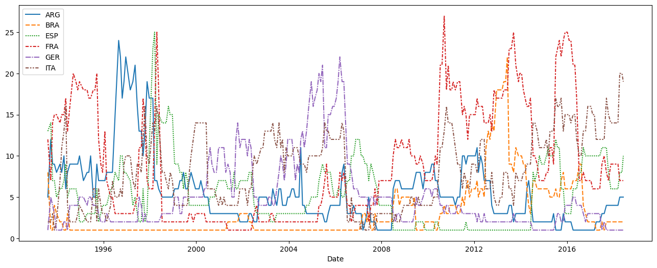

This code shouldn't make sense just yet, and you'll learn more about it in the upcoming tutorials. For now, continue to your first exercise, where you'll get a chance to experiment with the coding environment yourself!

这段代码目前还没有意义，您将在接下来的教程中了解更多信息。 现在，继续您的第一个练习，您将有机会亲自尝试编码环境！

What's next?

下一步是什么？

Write your first lines of code in the first coding exercise!

在 第一次编码练习 中编写您的第一行代码！