In this tutorial you'll learn all about histograms and density plots.

在本教程中，您将了解直方图和密度图的所有内容。

Set up the notebook

设置笔记本

As always, we begin by setting up the coding environment. (This code is hidden, but you can un-hide it by clicking on the "Code" button immediately below this text, on the right.)

与往常一样，我们首先设置编码环境。 （此代码已隐藏，但您可以通过单击该文本右侧紧邻的“代码”按钮来取消隐藏它。）

import pandas as pd
pd.plotting.register_matplotlib_converters()
import matplotlib.pyplot as plt
%matplotlib inline
import seaborn as sns
print("Setup Complete")

Setup Complete

Select a dataset

选择一个数据集

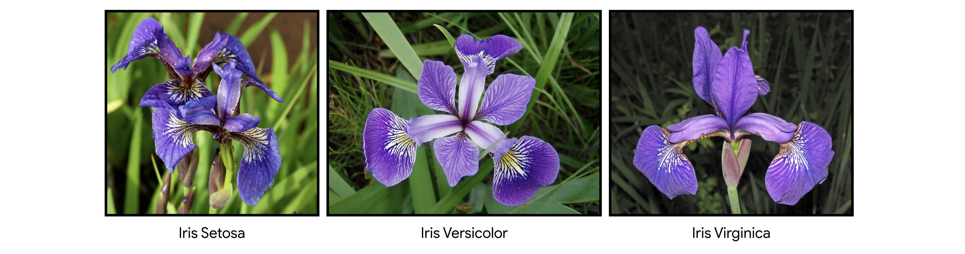
We'll work with a dataset of 150 different flowers, or 50 each from three different species of iris (Iris setosa, Iris versicolor, and Iris virginica).

我们将使用包含 150 种不同花朵的数据集，或者三种不同鸢尾花各 50 种（山鸢尾、变色鸢尾和维吉尼亚鸢尾）。

Load and examine the data

加载并检查数据

Each row in the dataset corresponds to a different flower. There are four measurements: the sepal length and width, along with the petal length and width. We also keep track of the corresponding species.

数据集中的每一行对应于不同的花。 有四种测量值：萼片长度和宽度，以及花瓣长度和宽度。 我们还跟踪相应的物种。

# Path of the file to read
iris_filepath = "../00 datasets/alexisbcook/data-for-datavis/iris.csv"

# Read the file into a variable iris_data
iris_data = pd.read_csv(iris_filepath, index_col="Id")

# Print the first 5 rows of the data
iris_data.head()

	Sepal Length (cm)	Sepal Width (cm)	Petal Length (cm)	Petal Width (cm)	Species
Id
1	5.1	3.5	1.4	0.2	Iris-setosa
2	4.9	3.0	1.4	0.2	Iris-setosa
3	4.7	3.2	1.3	0.2	Iris-setosa
4	4.6	3.1	1.5	0.2	Iris-setosa
5	5.0	3.6	1.4	0.2	Iris-setosa

Histograms

直方图

Say we would like to create a histogram to see how petal length varies in iris flowers. We can do this with the sns.histplot command.

假设我们想创建一个直方图来查看鸢尾花的花瓣长度如何变化。 我们可以使用sns.histplot命令来完成此操作。

# Histogram 
sns.histplot(iris_data['Petal Length (cm)'])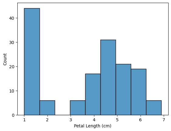

In the code cell above, we had to supply the command with the column we'd like to plot (_in this case, we chose MARKDOWN_HASH2339b4fb479c4a6f9844e3c85179263fMARKDOWNHASH).

在上面的代码单元中，我们必须为命令提供我们想要绘制的列（ _在本例中，我们选择MARKDOWN_HASHe00f01b1b60d47e209ab85ef10d19c14MARKDOWNHASH ）。

Density plots

密度图

The next type of plot is a kernel density estimate (KDE) plot. In case you're not familiar with KDE plots, you can think of it as a smoothed histogram.

下一种类型的图是核密度估计 (KDE) 图。 如果您不熟悉 KDE 图，您可以将其视为平滑直方图。

To make a KDE plot, we use the sns.kdeplot command. Setting shade=True colors the area below the curve (_and MARKDOWN_HASHd88654f7927666a02d8a5bd5104c5897MARKDOWNHASH chooses the column we would like to plot).

为了制作 KDE 绘图，我们使用 sns.kdeplot 命令。 设置shade=True为曲线下方的区域着色（ _并且MARKDOWN_HASHd88654f7927666a02d8a5bd5104c5897MARKDOWNHASH选择我们想要绘制的列 ）。

# KDE plot 
# sns.kdeplot(data=iris_data['Petal Length (cm)'], shade=True)
sns.kdeplot(data=iris_data['Petal Length (cm)'], fill=True)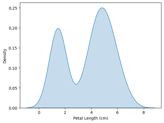

2D KDE plots

2D KDE 图

We're not restricted to a single column when creating a KDE plot. We can create a two-dimensional (2D) KDE plot with the sns.jointplot command.

创建 KDE 图时，我们不限于单列。 我们可以使用sns.jointplot命令创建二维 (2D) KDE 图。

In the plot below, the color-coding shows us how likely we are to see different combinations of sepal width and petal length, where darker parts of the figure are more likely.

在下图中，颜色编码向我们展示了我们看到萼片宽度和花瓣长度的不同组合的可能性有多大，其中图中较暗的部分更有可能出现。

# 2D KDE plot
sns.jointplot(x=iris_data['Petal Length (cm)'], y=iris_data['Sepal Width (cm)'], kind="kde")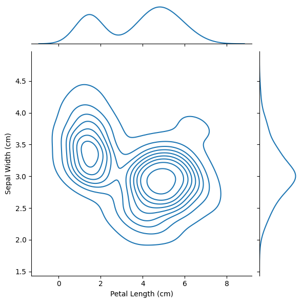

Note that in addition to the 2D KDE plot in the center,

请注意，除了中心的 2D KDE 图之外，

• the curve at the top of the figure is a KDE plot for the data on the x-axis (in this case, iris_data['Petal Length (cm)']), and
• 图顶部的曲线是 x 轴上数据的 KDE 图（在本例中为iris_data['Petal Length (cm)']），以及
• the curve on the right of the figure is a KDE plot for the data on the y-axis (in this case, iris_data['Sepal Width (cm)']).
• 图右侧的曲线是 y 轴数据的 KDE 图（在本例中为 iris_data['Sepal Width (cm)']）。

Color-coded plots

颜色编码图

For the next part of the tutorial, we'll create plots to understand differences between the species.

在本教程的下一部分中，我们将创建绘图来了解物种之间的差异。

We can create three different histograms (one for each species) of petal length by using the sns.histplot command (as above).

我们可以使用 sns.histplot 命令（如上所述）创建三个不同的花瓣长度直方图（每个物种一个）。

• data= provides the name of the variable that we used to read in the data
• data= 提供我们用来读取数据的变量的名称
• x= sets the name of column with the data we want to plot
• x= 设置包含我们想要绘制的数据的列的名称
• hue= sets the column we'll use to split the data into different histograms
• hue= 设置我们将用来将数据分割成不同直方图的列

# Histograms for each species
sns.histplot(data=iris_data, x='Petal Length (cm)', hue='Species')

# Add title
plt.title("Histogram of Petal Lengths, by Species")

Text(0.5, 1.0, 'Histogram of Petal Lengths, by Species')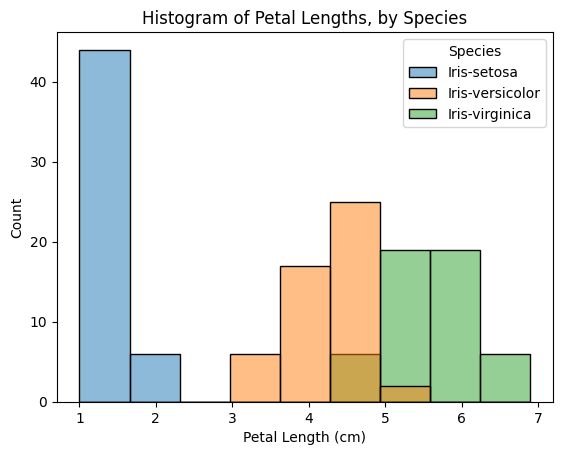

We can also create a KDE plot for each species by using sns.kdeplot (as above). The functionality for data, x, and hue are identical to when we used sns.histplot above. Additionally, we set shade=True to color the area below each curve.

我们还可以使用sns.kdeplot（ 如上所述 ）为每个种类创建 KDE 图。 data、x和hue的功能与我们上面使用sns.histplot时相同。 此外，我们设置shade=True来为每条曲线下方的区域着色。

# KDE plots for each species
# sns.kdeplot(data=iris_data, x='Petal Length (cm)', hue='Species', shade=True)
sns.kdeplot(data=iris_data, x='Petal Length (cm)', hue='Species', fill=True)

# Add title
plt.title("Distribution of Petal Lengths, by Species")

Text(0.5, 1.0, 'Distribution of Petal Lengths, by Species')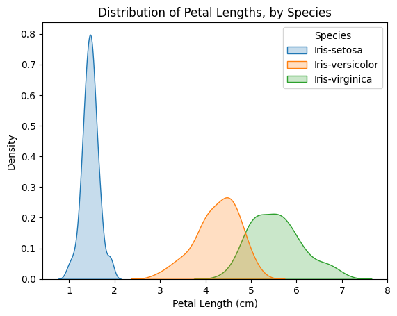

One interesting pattern that can be seen in plots is that the plants seem to belong to one of two groups, where Iris versicolor and Iris virginica seem to have similar values for petal length, while Iris setosa belongs in a category all by itself.

图中可以看到的一个有趣的模式是，这些植物似乎属于两个类群之一，其中 Iris versicolor 和 Iris virginica 似乎具有相似的花瓣长度值，而 Iris setosa 本身属于一个类别。

In fact, according to this dataset, we might even be able to classify any iris plant as Iris setosa (as opposed to Iris versicolor or Iris virginica) just by looking at the petal length: if the petal length of an iris flower is less than 2 cm, it's most likely to be Iris setosa!

事实上，根据这个数据集，我们甚至可以通过查看花瓣长度将任何鸢尾植物分类为 Iris setosa（而不是 Iris versicolor 或 Iris virginica）：如果花瓣长度 一朵小于2厘米的鸢尾花，很可能是Iris setosa！

What's next?

下一步是什么？

Put your new skills to work in a coding exercise!

将您的新技能运用到 编码练习！