Introduction

介绍

Once you've identified a set of features with some potential, it's time to start developing them. In this lesson, you'll learn a number of common transformations you can do entirely in Pandas. If you're feeling rusty, we've got a great course on Pandas.

一旦您确定了一组具有一定潜力的特征，就可以开始开发它们了。在本课程中，您将学习一些完全可以在 Pandas 中完成的常见转换。如果您感到生疏，我们有一个很棒的Pandas 课程。

We'll use four datasets in this lesson having a range of feature types: US Traffic Accidents, 1985 Automobiles, Concrete Formulations, and Customer Lifetime Value. The following hidden cell loads them up.

我们将在本课程中使用四个具有一系列特征类型的数据集：美国交通事故、 1985 汽车, 具体配方, 和 客户终身价值。以下隐藏单元格加载它们。


import matplotlib.pyplot as plt
import numpy as np
import pandas as pd
import seaborn as sns

plt.style.use("seaborn-v0_8-whitegrid")
plt.rc("figure", autolayout=True)
plt.rc(
    "axes",
    labelweight="bold",
    labelsize="large",
    titleweight="bold",
    titlesize=14,
    titlepad=10,
)

accidents = pd.read_csv("../00 datasets/ryanholbrook/fe-course-data/accidents.csv")
autos = pd.read_csv("../00 datasets/ryanholbrook/fe-course-data/autos.csv")
concrete = pd.read_csv("../00 datasets/ryanholbrook/fe-course-data/concrete.csv")
customer = pd.read_csv("../00 datasets/ryanholbrook/fe-course-data/customer.csv")

Tips on Discovering New Features
发现新功能的技巧

Understand the features. Refer to your dataset's data documentation, if available.

了解特征。请参阅数据集的数据文档（如果有）。

Research the problem domain to acquire domain knowledge. If your problem is predicting house prices, do some research on real-estate for instance. Wikipedia can be a good starting point, but books and journal articles will often have the best information.

研究问题领域以获得领域知识。如果您的问题是预测房价，请对房地产进行一些研究。维基百科可能是一个很好的起点，但书籍和期刊文章通常会提供最好的信息。

Study previous work. Solution write-ups from past Kaggle competitions are a great resource.

研究以前的工作。过去 Kaggle 竞赛的解决方案文章是一个很好的资源。

Use data visualization. Visualization can reveal pathologies in the distribution of a feature or complicated relationships that could be simplified. Be sure to visualize your dataset as you work through the feature engineering process.

使用数据可视化。可视化可以揭示特征分布的病态或可以简化的复杂关系。在完成特征工程过程时，请务必可视化您的数据集。

Mathematical Transforms

数学变换

Relationships among numerical features are often expressed through mathematical formulas, which you'll frequently come across as part of your domain research. In Pandas, you can apply arithmetic operations to columns just as if they were ordinary numbers.

数字特征之间的关系通常通过数学公式来表达，您在领域研究中经常会遇到这些公式。在 Pandas 中，您可以对列应用算术运算，就像它们是普通数字一样。

In the Automobile dataset are features describing a car's engine. Research yields a variety of formulas for creating potentially useful new features. The "stroke ratio", for instance, is a measure of how efficient an engine is versus how performant:

汽车数据集中是描述汽车发动机的特征。研究产生了各种用于创建潜在有用的新功能的公式。例如，“冲程比”是衡量发动机效率与性能的指标：

autos["stroke_ratio"] = autos.stroke / autos.bore

autos[["stroke", "bore", "stroke_ratio"]].head()

	stroke	bore	stroke_ratio
0	2.68	3.47	0.772334
1	2.68	3.47	0.772334
2	3.47	2.68	1.294776
3	3.40	3.19	1.065831
4	3.40	3.19	1.065831

The more complicated a combination is, the more difficult it will be for a model to learn, like this formula for an engine's "displacement", a measure of its power:

组合越复杂，模型学习就越困难，就像发动机“排量”（衡量其功率的指标）的公式一样：

autos["displacement"] = (
    np.pi * ((0.5 * autos.bore) ** 2) * autos.stroke * autos.num_of_cylinders
)

Data visualization can suggest transformations, often a "reshaping" of a feature through powers or logarithms. The distribution of WindSpeed in US Accidents is highly skewed, for instance. In this case the logarithm is effective at normalizing it:

数据可视化可以给出转换的建议，通常是通过幂或对数重塑特征。例如，WindSpeed在美国事故中的分布是高度倾斜的。在这种情况下，对数可以有效地对其进行标准化：

# If the feature has 0.0 values, use np.log1p (log(1+x)) instead of np.log
accidents["LogWindSpeed"] = accidents.WindSpeed.apply(np.log1p)

# Plot a comparison
fig, axs = plt.subplots(1, 2, figsize=(8, 4))
sns.kdeplot(accidents.WindSpeed, fill=True, ax=axs[0])
sns.kdeplot(accidents.LogWindSpeed, fill=True, ax=axs[1]);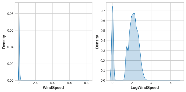

png

Check out our lesson on normalization in Data Cleaning where you'll also learn about the Box-Cox transformation, a very general kind of normalizer.

查看我们在数据清理中的标准化课程，您还将了解 Box-Cox 变换，这是一种非常通用的标准化器。

Counts

计数

Features describing the presence or absence of something often come in sets, the set of risk factors for a disease, say. You can aggregate such features by creating a count.

描述某种事物存在或不存在的特征通常是成组出现的，例如疾病的一组危险因素。您可以通过创建计数来聚合此类功能。

These features will be binary (1 for Present, 0 for Absent) or boolean (True or False). In Python, booleans can be added up just as if they were integers.

这些特征将是二进制（1表示存在，0表示不存在）或布尔（True或False）。在 Python 中，布尔值可以像整数一样相加。

In Traffic Accidents are several features indicating whether some roadway object was near the accident. This will create a count of the total number of roadway features nearby using the sum method:

在交通事故中，有几个特征指示事故附近是否存在某些道路物体。这将使用sum方法创建附近道路要素总数的计数：

roadway_features = ["Amenity", "Bump", "Crossing", "GiveWay",
    "Junction", "NoExit", "Railway", "Roundabout", "Station", "Stop",
    "TrafficCalming", "TrafficSignal"]
accidents["RoadwayFeatures"] = accidents[roadway_features].sum(axis=1)

accidents[roadway_features + ["RoadwayFeatures"]].head(10)

	Amenity	Bump	Crossing	GiveWay	Junction	NoExit	Railway	Roundabout	Station	Stop	TrafficCalming	TrafficSignal	RoadwayFeatures
0	False	False	False	False	False	False	False	False	False	False	False	False	0
1	False	False	False	False	False	False	False	False	False	False	False	False	0
2	False	False	False	False	False	False	False	False	False	False	False	False	0
3	False	False	False	False	False	False	False	False	False	False	False	False	0
4	False	False	False	False	False	False	False	False	False	False	False	False	0
5	False	False	False	False	True	False	False	False	False	False	False	False	1
6	False	False	False	False	False	False	False	False	False	False	False	False	0
7	False	False	True	False	False	False	False	False	False	False	False	True	2
8	False	False	True	False	False	False	False	False	False	False	False	True	2
9	False	False	False	False	False	False	False	False	False	False	False	False	0

You could also use a dataframe's built-in methods to create boolean values. In the Concrete dataset are the amounts of components in a concrete formulation. Many formulations lack one or more components (that is, the component has a value of 0). This will count how many components are in a formulation with the dataframe's built-in greater-than gt method:

您还可以使用dataframe的内置方法来创建布尔值。 混凝土 数据集中是混凝土配方中成分的数量。许多配方缺少一种或多种成分（即成分值为 0）。这将使用数据框的内置大于gt方法来计算配方中有多少个成分：

components = [ "Cement", "BlastFurnaceSlag", "FlyAsh", "Water",
               "Superplasticizer", "CoarseAggregate", "FineAggregate"]
concrete["Components"] = concrete[components].gt(0).sum(axis=1)

concrete[components + ["Components"]].head(10)

	Cement	BlastFurnaceSlag	Water	Superplasticizer	CoarseAggregate	FineAggregate	Components
0	540.0	0.0	162.0	2.5	1040.0	676.0	5
1	540.0	0.0	162.0	2.5	1055.0	676.0	5
2	332.5	142.5	228.0	0.0	932.0	594.0	5
3	332.5	142.5	228.0	0.0	932.0	594.0	5
4	198.6	132.4	192.0	0.0	978.4	825.5	5
5	266.0	114.0	228.0	0.0	932.0	670.0	5
6	380.0	95.0	228.0	0.0	932.0	594.0	5
7	380.0	95.0	228.0	0.0	932.0	594.0	5
8	266.0	114.0	228.0	0.0	932.0	670.0	5
9	475.0	0.0	228.0	0.0	932.0	594.0	4

Building-Up and Breaking-Down Features

构建和分解特征

Often you'll have complex strings that can usefully be broken into simpler pieces. Some common examples:

通常，您会拥有复杂的字符串，可以将其有效地分解为更简单的部分。一些常见的例子：

ID numbers: '123-45-6789'
身份证号码：123-45-6789
Phone numbers: '(999) 555-0123'
电话号码：(999) 555-0123
Street addresses: '8241 Kaggle Ln., Goose City, NV'
街道地址：8241 Kaggle Ln., Goose City, NV
Internet addresses: 'http://www.kaggle.com
互联网地址：http://www.kaggle.com
Product codes: '0 36000 29145 2'
产品代码：0 36000 29145 2
Dates and times: 'Mon Sep 30 07:06:05 2013'
日期和时间：2013 年 9 月 30 日星期一 07:06:05

Features like these will often have some kind of structure that you can make use of. US phone numbers, for instance, have an area code (the '(999)' part) that tells you the location of the caller. As always, some research can pay off here.

此类特征通常具有某种可供您使用的结构。例如，美国的电话号码有一个区号（(999)部分），可以告诉您呼叫者的位置。一如既往，一些研究可以在这里得到有用的信息。

The str accessor lets you apply string methods like split directly to columns. The Customer Lifetime Value dataset contains features describing customers of an insurance company. From the Policy feature, we could separate the Type from the Level of coverage:

str 访问器允许您将 split 等字符串方法直接应用于列。 客户终身价值 数据集包含描述保险公司客户的特征。从策略特征中，我们可以将覆盖范围的类型与级别分开：

customer[["Type", "Level"]] = (  # Create two new features
    customer["Policy"]           # from the Policy feature
    .str                         # through the string accessor
    .split(" ", expand=True)     # by splitting on " "
                                 # and expanding the result into separate columns
)

customer[["Policy", "Type", "Level"]].head(10)

	Policy	Type	Level
0	Corporate L3	Corporate	L3
1	Personal L3	Personal	L3
2	Personal L3	Personal	L3
3	Corporate L2	Corporate	L2
4	Personal L1	Personal	L1
5	Personal L3	Personal	L3
6	Corporate L3	Corporate	L3
7	Corporate L3	Corporate	L3
8	Corporate L3	Corporate	L3
9	Special L2	Special	L2

You could also join simple features into a composed feature if you had reason to believe there was some interaction in the combination:

如果您有理由相信组合中存在一些关联，您也可以将简单特征加入到组合特征中：

autos["make_and_style"] = autos["make"] + "_" + autos["body_style"]
autos[["make", "body_style", "make_and_style"]].head()

	make	body_style	make_and_style
0	alfa-romero	convertible	alfa-romero_convertible
1	alfa-romero	convertible	alfa-romero_convertible
2	alfa-romero	hatchback	alfa-romero_hatchback
3	audi	sedan	audi_sedan
4	audi	sedan	audi_sedan

Elsewhere on Kaggle Learn
Kaggle Learn 上的其他地方

There are a few other kinds of data we haven't talked about here that are especially rich in information. Fortunately, we've got you covered!

还有一些我们在这里没有讨论的其他类型的数据，它们的信息特别丰富。幸运的是，我们已经为您提供了保障！

For dates and times, see Parsing Dates from our Data Cleaning course.

对于日期和时间，请参阅我们的数据清理课程中的解析日期。

For latitudes and longitudes, see our Geospatial Analysis course.

对于纬度和经度，请参阅我们的地理空间分析课程。

Group Transforms

组变换

Finally we have Group transforms, which aggregate information across multiple rows grouped by some category. With a group transform you can create features like: "the average income of a person's state of residence," or "the proportion of movies released on a weekday, by genre." If you had discovered a category interaction, a group transform over that categry could be something good to investigate.

最后，我们有组转换，它聚合按某个类别分组的多行信息。通过组转换，您可以创建诸如一个人居住州的平均收入或按类型在工作日发行的电影的比例等功能。如果您发现了类别交互，那么针对该类别的组转换可能是值得研究的好东西。

Using an aggregation function, a group transform combines two features: a categorical feature that provides the grouping and another feature whose values you wish to aggregate. For an "average income by state", you would choose State for the grouping feature, mean for the aggregation function, and Income for the aggregated feature. To compute this in Pandas, we use the groupby and transform methods:

使用聚合函数，组转换组合了两个特征：一个提供分组的分类特征和另一个要聚合其值的特征。对于按州划分的平均收入，您可以选择State作为分组特征，选择mean作为聚合函数，选择Income作为聚合特征。为了在 Pandas 中计算这个，我们使用groupby和transform方法：

customer["AverageIncome"] = (
    customer.groupby("State")  # for each state
    ["Income"]                 # select the income
    .transform("mean")         # and compute its mean
)

customer[["State", "Income", "AverageIncome"]].head(10)

	State	Income	AverageIncome
0	Washington	56274	38122.733083
1	Arizona	0	37405.402231
2	Nevada	48767	38369.605442
3	California	0	37558.946667
4	Washington	43836	38122.733083
5	Oregon	62902	37557.283353
6	Oregon	55350	37557.283353
7	Arizona	0	37405.402231
8	Oregon	14072	37557.283353
9	Oregon	28812	37557.283353

The mean function is a built-in dataframe method, which means we can pass it as a string to transform. Other handy methods include max, min, median, var, std, and count. Here's how you could calculate the frequency with which each state occurs in the dataset:

mean函数是一个内置的Dataframe方法，这意味着我们可以将其作为字符串传递给transform。其他方便的方法包括max、min、median、var、std和count。以下是计算数据集中每个状态出现的频率的方法：

customer["StateFreq"] = (
    customer.groupby("State")
    ["State"]
    .transform("count")
    / customer.State.count()
)

customer[["State", "StateFreq"]].head(10)

	State	StateFreq
0	Washington	0.087366
1	Arizona	0.186446
2	Nevada	0.096562
3	California	0.344865
4	Washington	0.087366
5	Oregon	0.284760
6	Oregon	0.284760
7	Arizona	0.186446
8	Oregon	0.284760
9	Oregon	0.284760

You could use a transform like this to create a "frequency encoding" for a categorical feature.

您可以使用这样的转换来为分类特征创建频率编码。

If you're using training and validation splits, to preserve their independence, it's best to create a grouped feature using only the training set and then join it to the validation set. We can use the validation set's merge method after creating a unique set of values with drop_duplicates on the training set:

如果您使用训练和验证拆分，为了保持它们的独立性，最好仅使用训练集创建分组特征，然后将其加入验证集。在训练集上使用drop_duplicates创建一组唯一的值后，我们可以使用验证集的merge方法：

# Create splits
df_train = customer.sample(frac=0.5)
df_valid = customer.drop(df_train.index)

# Create the average claim amount by coverage type, on the training set
df_train["AverageClaim"] = df_train.groupby("Coverage")["ClaimAmount"].transform("mean")

# Merge the values into the validation set
df_valid = df_valid.merge(
    df_train[["Coverage", "AverageClaim"]].drop_duplicates(),
    on="Coverage",
    how="left",
)

df_valid[["Coverage", "AverageClaim"]].head(10)

	Coverage	AverageClaim
0	Basic	384.381665
1	Basic	384.381665
2	Basic	384.381665
3	Premium	647.709408
4	Basic	384.381665
5	Extended	492.302996
6	Premium	647.709408
7	Basic	384.381665
8	Basic	384.381665
9	Basic	384.381665

Tips on Creating Features
创建特征的技巧

It's good to keep in mind your model's own strengths and weaknesses when creating features. Here are some guidelines:
创建特征时最好记住模型自身的优点和缺点。以下是一些准则：

Linear models learn sums and differences naturally, but can't learn anything more complex.

线性模型自然地学习和与差，但无法学习更复杂的东西。

Ratios seem to be difficult for most models to learn. Ratio combinations often lead to some easy performance gains.

对于大多数模型来说，比率似乎很难学习。组合比率通常会带来一些简单的性能提升。

Linear models and neural nets generally do better with normalized features. Neural nets especially need features scaled to values not too far from 0. Tree-based models (like random forests and XGBoost) can sometimes benefit from normalization, but usually much less so.

线性模型和神经网络通常在归一化特征方面表现更好。神经网络特别需要缩放到离 0 不太远的值的特征。基于树的模型（如随机森林和 XGBoost）有时可以从归一化中受益，但通常效果要差得多。

Tree models can learn to approximate almost any combination of features, but when a combination is especially important they can still benefit from having it explicitly created, especially when data is limited.

树模型可以学习近似任何特征组合，但是当组合特别重要时，它们仍然可以从显式创建的组合中受益，特别是当数据有限时。

Counts are especially helpful for tree models, since these models don't have a natural way of aggregating information across many features at once.

计数对于树模型特别有用，因为这些模型没有一种自然的方式来同时聚合多个特征的信息。

Your Turn

到你了

Combine and transform features from Ames and improve your model's performance.

针对 Ames 组合和转换功能，并提高模型的性能。

03.course-creating-features【创建特征】