Introduction

介绍

This lesson and the next make use of what are known as unsupervised learning algorithms. Unsupervised algorithms don't make use of a target; instead, their purpose is to learn some property of the data, to represent the structure of the features in a certain way. In the context of feature engineering for prediction, you could think of an unsupervised algorithm as a "feature discovery" technique.

本课和下一课将使用所谓的无监督学习算法。 无监督算法不利用目标； 相反，它们的目的是学习数据的某些属性，以某种方式表示特征的结构。 在为进行预测进行的特征工程背景下，您可以将无监督算法视为特征发现技术。

Clustering simply means the assigning of data points to groups based upon how similar the points are to each other. A clustering algorithm makes "birds of a feather flock together," so to speak.

聚类简单地意味着根据数据点彼此之间的相似程度将数据点分配到组中。 可以说，聚类算法使物以类聚。

When used for feature engineering, we could attempt to discover groups of customers representing a market segment, for instance, or geographic areas that share similar weather patterns. Adding a feature of cluster labels can help machine learning models untangle complicated relationships of space or proximity.

例如，当用于特征工程时，我们可以尝试发现代表细分市场的客户群体，或具有相似天气模式的地理区域。 添加集群标签的功能可以帮助机器学习模型理清复杂的空间或邻近关系。

Cluster Labels as a Feature

聚类标签作为特征

Applied to a single real-valued feature, clustering acts like a traditional "binning" or "discretization" transform. On multiple features, it's like "multi-dimensional binning" (sometimes called vector quantization).

应用于单个实值特征时，聚类的作用类似于传统的分箱或离散化变换。 在多个特征上，它就像多维分箱（有时称为矢量量化）。

Left: Clustering a single feature. Right: Clustering across two features.
左：对单个特征进行聚类。 右：跨两个特征进行聚类。

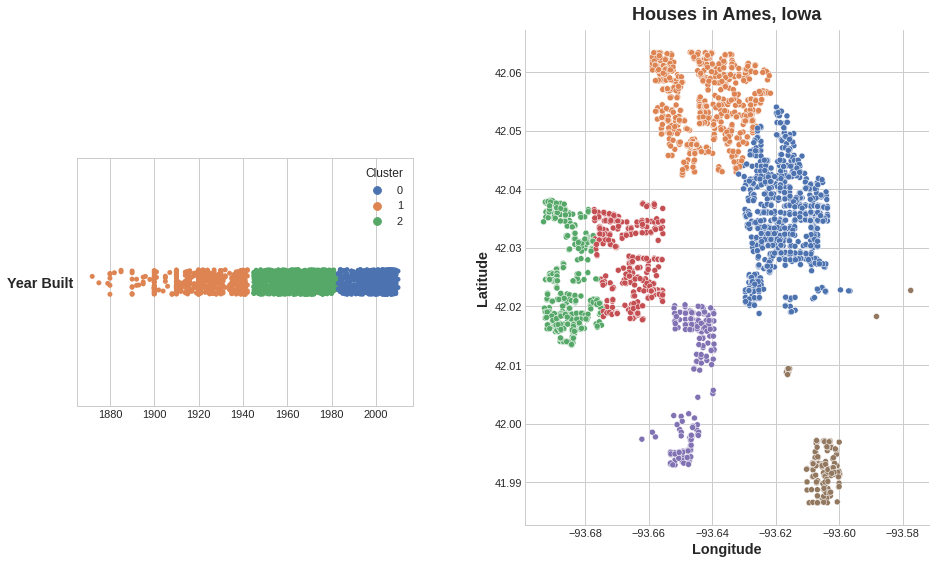
Added to a dataframe, a feature of cluster labels might look like this:

添加到dataframe中，集群标签的特征可能如下所示：

Longitude	Latitude	Cluster
-93.619	42.054	3
-93.619	42.053	3
-93.638	42.060	1
-93.602	41.988	0

It's important to remember that this Cluster feature is categorical. Here, it's shown with a label encoding (that is, as a sequence of integers) as a typical clustering algorithm would produce; depending on your model, a one-hot encoding may be more appropriate.

重要的是要记住，这个集群特征是有类别的。 在这里，它显示为标签编码（即，作为整数序列），如典型的聚类算法所产生的那样； 根据您的模型，one-hot 编码可能更合适。

The motivating idea for adding cluster labels is that the clusters will break up complicated relationships across features into simpler chunks. Our model can then just learn the simpler chunks one-by-one instead having to learn the complicated whole all at once. It's a "divide and conquer" strategy.

添加集群标签的动机是集群会将特征之间的复杂关系分解为更简单的块。 然后，我们的模型可以一个个的学习更简单的块，而不必一次学习复杂的整体。 这是一种分而治之的策略。

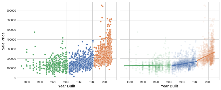
The figure shows how clustering can improve a simple linear model. The curved relationship between the YearBuilt and SalePrice is too complicated for this kind of model -- it underfits. On smaller chunks however the relationship is almost linear, and that the model can learn easily.

该图显示了聚类如何改进简单的线性模型。 对于这种模型来说，YearBuilt和SalePrice之间的曲线关系过于复杂——它是欠拟合的。 然而，在较小的块上，关系几乎是线性的，并且模型可以轻松学习。

k-Means Clustering

k 均值聚类

There are a great many clustering algorithms. They differ primarily in how they measure "similarity" or "proximity" and in what kinds of features they work with. The algorithm we'll use, k-means, is intuitive and easy to apply in a feature engineering context. Depending on your application another algorithm might be more appropriate.

聚类算法有很多。 它们的不同之处主要在于如何使用哪些类型的特征来衡量相似性或接近程度。 我们将使用的算法 k-means 非常直观且易于在特征工程环境中应用。 根据您的应用程序，另一种算法可能更合适。

K-means clustering measures similarity using ordinary straight-line distance (Euclidean distance, in other words). It creates clusters by placing a number of points, called centroids, inside the feature-space. Each point in the dataset is assigned to the cluster of whichever centroid it's closest to. The "k" in "k-means" is how many centroids (that is, clusters) it creates. You define the k yourself.

K-means 聚类 使用普通直线距离（换句话说，欧几里得距离）来测量相似性。 它通过在特征空间内放置许多点（称为质心）来创建簇。 数据集中的每个点都分配给最接近的质心的簇。 k-means中的k是它创建的质心（即簇）数量。 您自己定义 k 值。

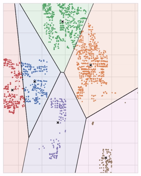
You could imagine each centroid capturing points through a sequence of radiating circles. When sets of circles from competing centroids overlap they form a line. The result is what's called a Voronoi tessallation. The tessallation shows you to what clusters future data will be assigned; the tessallation is essentially what k-means learns from its training data.

您可以想象每个质心通过一系列辐射圆捕获点。 当来自竞争质心的圆组重叠时，它们会形成一条线。 结果就是所谓的 Voronoi 镶嵌。 镶嵌会向您显示未来数据将分配到哪些集群； 镶嵌本质上是 k-means 从训练数据中学习的内容。

The clustering on the Ames dataset above is a k-means clustering. Here is the same figure with the tessallation and centroids shown.

上面的 Ames 数据集上的聚类是 k 均值聚类。 这是同一张图，显示了镶嵌和质心。

Let's review how the k-means algorithm learns the clusters and what that means for feature engineering. We'll focus on three parameters from scikit-learn's implementation: n_clusters, max_iter, and n_init.

让我们回顾一下 k 均值算法如何学习聚类以及这对特征工程意味着什么。 我们将重点关注 scikit-learn 实现中的三个参数：n_clusters、max_iter和n_init。

It's a simple two-step process. The algorithm starts by randomly initializing some predefined number (n_clusters) of centroids. It then iterates over these two operations:

这是一个简单的两步过程。 该算法首先随机初始化一些预定义数量（n_clusters）的质心。 然后它迭代这两个操作：

1. assign points to the nearest cluster centroid
2. 将点分配给最近的簇质心
3. move each centroid to minimize the distance to its points
4. 移动每个质心以最小化到其点的距离

It iterates over these two steps until the centroids aren't moving anymore, or until some maximum number of iterations has passed (max_iter).

它迭代这两个步骤，直到质心不再移动，或者直到经过了最大迭代次数（max_iter）。

It often happens that the initial random position of the centroids ends in a poor clustering. For this reason the algorithm repeats a number of times (n_init) and returns the clustering that has the least total distance between each point and its centroid, the optimal clustering.

质心的初始随机位置经常以较差的聚类结束。 因此，该算法会重复多次（n_init）并返回每个点与其质心之间总距离最小的聚类，即最佳聚类。

The animation below shows the algorithm in action. It illustrates the dependence of the result on the initial centroids and the importance of iterating until convergence.

下面的动画显示了正在运行的算法。 它说明了结果对初始质心的依赖性以及迭代直至收敛的重要性。

You may need to increase the max_iter for a large number of clusters or n_init for a complex dataset. Ordinarily though the only parameter you'll need to choose yourself is n_clusters (k, that is). The best partitioning for a set of features depends on the model you're using and what you're trying to predict, so it's best to tune it like any hyperparameter (through cross-validation, say).

您可能需要为大量集群增加max_iter，或为复杂数据集增加n_init。 通常，您需要自己选择的唯一参数是n_clusters（即 k）。 一组特征的最佳划分取决于您正在使用的模型以及您想要预测的内容，因此最好像任何超参数一样对其进行调整（例如通过交叉验证）。

Example - California Housing

示例 - 加州住房

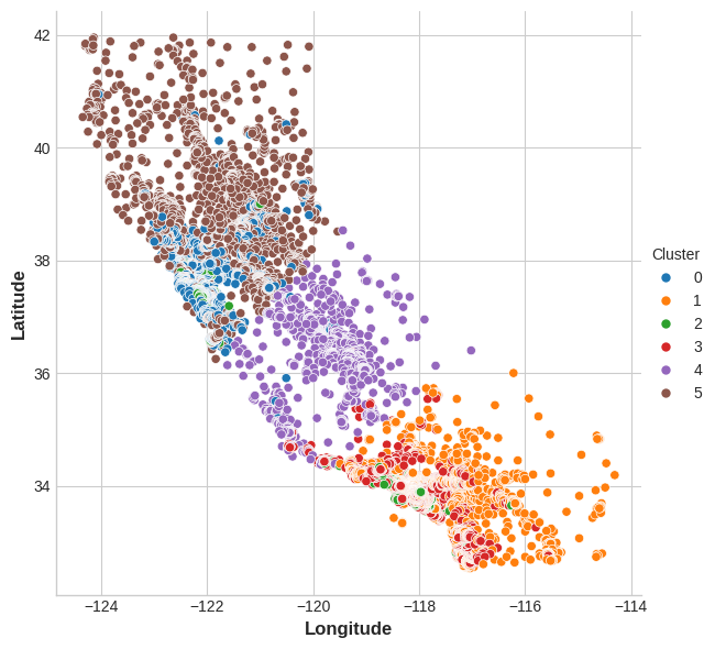
As spatial features, California Housing's 'Latitude' and 'Longitude' make natural candidates for k-means clustering. In this example we'll cluster these with 'MedInc' (median income) to create economic segments in different regions of California.

作为空间特征，加州住房 的纬度和经度自然成为 k 均值聚类的候选者 。 在此示例中，我们将这些与MedInc（收入中位数）聚集在一起，以在加利福尼亚州的不同地区创建经济细分。

import matplotlib.pyplot as plt
import pandas as pd
import seaborn as sns
from sklearn.cluster import KMeans

plt.style.use("seaborn-v0_8-whitegrid")
# plt.style.use("grayscale")
plt.rc("figure", autolayout=True)
plt.rc(
    "axes",
    labelweight="bold",
    labelsize="large",
    titleweight="bold",
    titlesize=14,
    titlepad=10,
)

df = pd.read_csv("../00 datasets/ryanholbrook/fe-course-data/housing.csv")
X = df.loc[:, ["MedInc", "Latitude", "Longitude"]]
X.head()

	MedInc	Latitude	Longitude
0	8.3252	37.88	-122.23
1	8.3014	37.86	-122.22
2	7.2574	37.85	-122.24
3	5.6431	37.85	-122.25
4	3.8462	37.85	-122.25

Since k-means clustering is sensitive to scale, it can be a good idea rescale or normalize data with extreme values. Our features are already roughly on the same scale, so we'll leave them as-is.

由于 k 均值聚类对规模很敏感，因此重新调整或标准化具有极值的数据可能是一个好主意。 我们的特征已经大致处于相同的规模，因此我们将保持原样。

# Create cluster feature
kmeans = KMeans(n_clusters=6)
X["Cluster"] = kmeans.fit_predict(X)
X["Cluster"] = X["Cluster"].astype("category")

X.head()

	MedInc	Latitude	Longitude	Cluster
0	8.3252	37.88	-122.23	0
1	8.3014	37.86	-122.22	0
2	7.2574	37.85	-122.24	0
3	5.6431	37.85	-122.25	0
4	3.8462	37.85	-122.25	5

Now let's look at a couple plots to see how effective this was. First, a scatter plot that shows the geographic distribution of the clusters. It seems like the algorithm has created separate segments for higher-income areas on the coasts.

现在让我们看几个图，看看这有多有效。 首先，散点图显示集群的地理分布。 该算法似乎为沿海高收入地区创建了单独的细分市场。

sns.relplot(
    x="Longitude", y="Latitude", hue="Cluster", data=X, height=6,
);

The target in this dataset is MedHouseVal (median house value). These box-plots show the distribution of the target within each cluster. If the clustering is informative, these distributions should, for the most part, separate across MedHouseVal, which is indeed what we see.

该数据集中的目标是MedHouseVal（房屋中位值）。 这些箱线图显示了每个簇内目标的分布。 如果聚类信息丰富，那么这些分布在大多数情况下应该在MedHouseVal中分离，这确实是我们所看到的。

X["MedHouseVal"] = df["MedHouseVal"]
sns.catplot(x="MedHouseVal", y="Cluster", data=X, kind="boxen", height=6);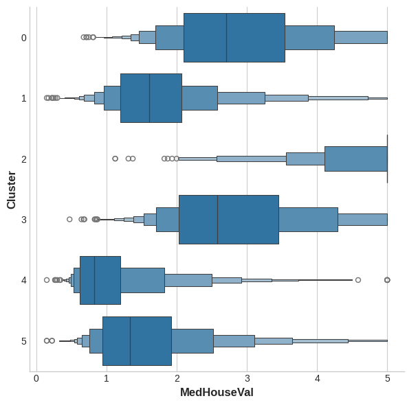

Your Turn

到你了

Add a feature of cluster labels to Ames and learn about another kind of feature clustering can create.

添加聚类标签特征到 Ames 数据集并了解聚类可以创建的另一种特征。