Introduction

介绍

In the previous lesson we looked at our first model-based method for feature engineering: clustering. In this lesson we look at our next: principal component analysis (PCA). Just like clustering is a partitioning of the dataset based on proximity, you could think of PCA as a partitioning of the variation in the data. PCA is a great tool to help you discover important relationships in the data and can also be used to create more informative features.

在上一课中，我们了解了第一个基于模型的特征工程方法：聚类。 在本课中，我们将学习下一课：主成分分析 (PCA)。 就像聚类是根据邻近度对数据集进行分区一样，您可以将 PCA 视为对数据变化的分区。 PCA 是一个很好的工具，可以帮助您发现数据中的重要关系，还可以用于创建信息更丰富的特征。

(Technical note: PCA is typically applied to standardized data. With standardized data "variation" means "correlation". With unstandardized data "variation" means "covariance". All data in this course will be standardized before applying PCA.)

（技术说明：PCA 通常应用于标准化 数据。对于标准化数据，“变化”意味着“相关性”。对于非标准化数据，“变化”意味着“协方差”。本课程中的所有数据将在应用 PCA 之前进行标准化。）

Principal Component Analysis

主成分分析

In the Abalone dataset are physical measurements taken from several thousand Tasmanian abalone. (An abalone is a sea creature much like a clam or an oyster.) We'll just look at a couple features for now: the 'Height' and 'Diameter' of their shells.

在 Abalone 数据集中，是对数千只塔斯马尼亚鲍鱼进行的物理测量。 （鲍鱼是一种海洋生物，很像蛤或牡蛎。）我们现在只看几个特征：壳的高度和直径。

You could imagine that within this data are "axes of variation" that describe the ways the abalone tend to differ from one another. Pictorially, these axes appear as perpendicular lines running along the natural dimensions of the data, one axis for each original feature.

您可以想象，这些数据中存在变异轴，描述了鲍鱼之间的差异。 从图中可以看出，这些轴显示为沿着数据的自然维度延伸的垂直线，每个原始特征对应一个轴。

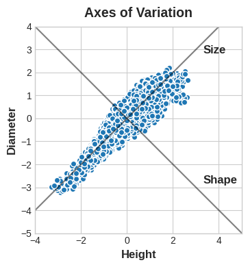
Often, we can give names to these axes of variation. The longer axis we might call the "Size" component: small height and small diameter (lower left) contrasted with large height and large diameter (upper right). The shorter axis we might call the "Shape" component: small height and large diameter (flat shape) contrasted with large height and small diameter (round shape).

通常，我们可以为这些变化轴命名。 较长的轴我们可以称为“尺寸”组件：小高度和小直径（左下）与大高度和大直径（右上）形成对比。 我们可以将较短的轴称为“形状”组件：小高度和大直径（扁平形状）与大高度和小直径（圆形）形成对比。

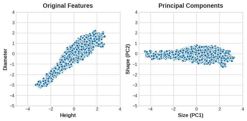
Notice that instead of describing abalones by their 'Height' and 'Diameter', we could just as well describe them by their 'Size' and 'Shape'. This, in fact, is the whole idea of PCA: instead of describing the data with the original features, we describe it with its axes of variation. The axes of variation become the new features.

请注意，我们不必通过高度和直径来描述鲍鱼，而是可以通过大小和形状来描述它们。 事实上，这就是 PCA 的全部思想：我们不是用原始特征来描述数据，而是用它的变化轴来描述它。 变化的轴成为新的特征。

The new features PCA constructs are actually just linear combinations (weighted sums) of the original features:

新特征 PCA 构造实际上只是原始特征的线性组合（加权和）：

df["Size"] = 0.707 * X["Height"] + 0.707 * X["Diameter"]
df["Shape"] = 0.707 * X["Height"] - 0.707 * X["Diameter"]

These new features are called the principal components of the data. The weights themselves are called loadings. There will be as many principal components as there are features in the original dataset: if we had used ten features instead of two, we would have ended up with ten components.

这些新特征称为数据的主成分。 权重本身称为载荷。 原始数据集中有多少个特征，就有多少个主成分：如果我们使用十个特征而不是两个，我们最终会得到十个成分。

A component's loadings tell us what variation it expresses through signs and magnitudes:

组件的载荷告诉我们它通过符号和大小表达的变化：

Features \ Components	Size (PC1)	Shape (PC2)
Height	0.707	0.707
Diameter	0.707	-0.707

This table of loadings is telling us that in the Size component, Height and Diameter vary in the same direction (same sign), but in the Shape component they vary in opposite directions (opposite sign). In each component, the loadings are all of the same magnitude and so the features contribute equally in both.

该载荷表告诉我们，在大小组件中，高度和直径沿相同方向变化（相同符号），但在形状组件中它们沿相反方向变化（相反符号）。 在每个组件中，载荷的大小都相同，因此特征在两个组件中的贡献相同。

PCA also tells us the amount of variation in each component. We can see from the figures that there is more variation in the data along the Size component than along the Shape component. PCA makes this precise through each component's percent of explained variance.

PCA 还告诉我们每个组件的变化量。 从图中我们可以看到，大小分量的数据变化比形状分量的数据变化更大。 PCA 通过每个组件的 解释方差百分比 使这一点变得精确。

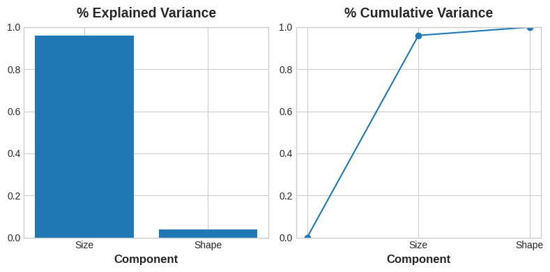
The Size component captures the majority of the variation between Height and Diameter. It's important to remember, however, that the amount of variance in a component doesn't necessarily correspond to how good it is as a predictor: it depends on what you're trying to predict.

尺寸组件捕获了高度和直径之间的大部分变化。 然而，重要的是要记住，组件中的方差量并不一定与其作为预测变量的效果相对应：它取决于您想要预测的内容。

PCA for Feature Engineering

用于特征工程的 PCA

There are two ways you could use PCA for feature engineering.

有两种方法可以使用 PCA 进行特征工程。

The first way is to use it as a descriptive technique. Since the components tell you about the variation, you could compute the MI scores for the components and see what kind of variation is most predictive of your target. That could give you ideas for kinds of features to create -- a product of 'Height' and 'Diameter' if 'Size' is important, say, or a ratio of 'Height' and 'Diameter' if Shape is important. You could even try clustering on one or more of the high-scoring components.

第一种方法是将其用作描述性技术。 由于组件会告诉您变化，因此您可以计算组件的 MI 分数，并查看哪种变化最能预测您的目标。 这可以为您提供创建各种特征的想法 - 如果尺寸很重要，则可以创建高度和直径的乘积，或者高度和直径的比率 如果形状很重要，则直径。 您甚至可以尝试对一个或多个高分组件进行聚类。

The second way is to use the components themselves as features. Because the components expose the variational structure of the data directly, they can often be more informative than the original features. Here are some use-cases:
第二种方法是使用组件本身作为特征。 由于组件直接暴露数据的变分结构，因此它们通常比原始特征提供更多信息。 以下是一些用例：

• Dimensionality reduction: When your features are highly redundant (multicollinear, specifically), PCA will partition out the redundancy into one or more near-zero variance components, which you can then drop since they will contain little or no information.
• 降维：当您的特征高度冗余时（特别是多重共线性），PCA 会将冗余划分为一个或多个接近零方差的分量，然后您可以将其删除，因为它们包含很少或不包含信息。
• Anomaly detection: Unusual variation, not apparent from the original features, will often show up in the low-variance components. These components could be highly informative in an anomaly or outlier detection task.
• 异常检测：原始特征中不明显的异常变化通常会出现在低方差组件中。 这些组件在异常或异常值检测任务中可能提供大量信息。
• Noise reduction: A collection of sensor readings will often share some common background noise. PCA can sometimes collect the (informative) signal into a smaller number of features while leaving the noise alone, thus boosting the signal-to-noise ratio.
• 降噪：传感器读数的集合通常会共享一些常见的背景噪声。 PCA 有时可以将（信息丰富的）信号收集到较少数量的特征中，同时保留噪声，从而提高信噪比。
• Decorrelation: Some ML algorithms struggle with highly-correlated features. PCA transforms correlated features into uncorrelated components, which could be easier for your algorithm to work with.
• 去相关：一些机器学习算法难以应对高度相关的特征。 PCA 将相关特征转换为不相关成分，这可以让您的算法更容易使用。

PCA basically gives you direct access to the correlational structure of your data. You'll no doubt come up with applications of your own!

PCA 基本上可以让您直接访问数据的相关结构。 毫无疑问，您会想出自己的应用程序！

PCA Best Practices
PCA 最佳实践

There are a few things to keep in mind when applying PCA:
应用PCA时需要记住以下几点：

• PCA only works with numeric features, like continuous quantities or counts.
• PCA 仅适用于数字特征，例如连续数量或计数。
• PCA is sensitive to scale. It's good practice to standardize your data before applying PCA, unless you know you have good reason not to.
• PCA 对规模敏感。 在应用 PCA 之前标准化您的数据是一个很好的做法，除非您知道有充分的理由不这样做。
• Consider removing or constraining outliers, since they can have an undue influence on the results.
• 考虑删除或限制异常值，因为它们可能会对结果产生不当影响。

Example - 1985 Automobiles

示例 - 1985 年汽车

In this example, we'll return to our Automobile dataset and apply PCA, using it as a descriptive technique to discover features. We'll look at other use-cases in the exercise.

在此示例中，我们将返回 Automobile 数据集并应用 PCA，将其用作发现特征的描述性技术。 我们将在练习中查看其他用例。

This hidden cell loads the data and defines the functions plot_variance and make_mi_scores.

该隐藏单元加载数据并定义函数plot_variance和make_mi_scores。

import matplotlib.pyplot as plt
import numpy as np
import pandas as pd
import seaborn as sns
from IPython.display import display
from sklearn.feature_selection import mutual_info_regression

plt.style.use("Solarize_Light2")
plt.rc("figure", autolayout=True)
plt.rc(
    "axes",
    labelweight="bold",
    labelsize="large",
    titleweight="bold",
    titlesize=14,
    titlepad=10,
)

def plot_variance(pca, width=8, dpi=100):
    # Create figure
    fig, axs = plt.subplots(1, 2)
    n = pca.n_components_
    grid = np.arange(1, n + 1)
    # Explained variance
    evr = pca.explained_variance_ratio_
    axs[0].bar(grid, evr)
    axs[0].set(
        xlabel="Component", title="% Explained Variance", ylim=(0.0, 1.0)
    )
    # Cumulative Variance
    cv = np.cumsum(evr)
    axs[1].plot(np.r_[0, grid], np.r_[0, cv], "o-")
    axs[1].set(
        xlabel="Component", title="% Cumulative Variance", ylim=(0.0, 1.0)
    )
    # Set up figure
    fig.set(figwidth=8, dpi=100)
    return axs

def make_mi_scores(X, y, discrete_features):
    mi_scores = mutual_info_regression(X, y, discrete_features=discrete_features)
    mi_scores = pd.Series(mi_scores, name="MI Scores", index=X.columns)
    mi_scores = mi_scores.sort_values(ascending=False)
    return mi_scores

df = pd.read_csv("../00 datasets/ryanholbrook/fe-course-data/autos.csv")

We've selected four features that cover a range of properties. Each of these features also has a high MI score with the target, price. We'll standardize the data since these features aren't naturally on the same scale.

我们选择了涵盖一系列属性的四个特征。 这些特征中的每一个都具有较高的 MI 分数，其目标是价格。 我们将对数据进行标准化，因为这些特征自然不在同一尺度上。

features = ["highway_mpg", "engine_size", "horsepower", "curb_weight"]

X = df.copy()
y = X.pop('price')
X = X.loc[:, features]

# Standardize
X_scaled = (X - X.mean(axis=0)) / X.std(axis=0)

Now we can fit scikit-learn's PCA estimator and create the principal components. You can see here the first few rows of the transformed dataset.

现在我们可以拟合 scikit-learn 的PCA估计器并创建主成分。 您可以在此处看到转换后的数据集的前几行。

from sklearn.decomposition import PCA

# Create principal components
pca = PCA()
X_pca = pca.fit_transform(X_scaled)

# Convert to dataframe
component_names = [f"PC{i+1}" for i in range(X_pca.shape[1])]
X_pca = pd.DataFrame(X_pca, columns=component_names)

X_pca.head()

	PC1	PC2	PC3	PC4
0	0.382486	-0.400222	0.124122	0.169539
1	0.382486	-0.400222	0.124122	0.169539
2	1.550890	-0.107175	0.598361	-0.256081
3	-0.408859	-0.425947	0.243335	0.013920
4	1.132749	-0.814565	-0.202885	0.224138

After fitting, the PCA instance contains the loadings in its components_ attribute. (Terminology for PCA is inconsistent, unfortunately. We're following the convention that calls the transformed columns in X_pca the components, which otherwise don't have a name.) We'll wrap the loadings up in a dataframe.

拟合后，PCA实例在其components_属性中包含载荷。 （不幸的是，PCA 的术语不一致。我们遵循将X_pca中转换后的列称为组件的约定，否则这些列没有名称。）我们将把加载包装在数据框中。

loadings = pd.DataFrame(
    pca.components_.T,  # transpose the matrix of loadings
    columns=component_names,  # so the columns are the principal components
    index=X.columns,  # and the rows are the original features
)
loadings

	PC1	PC2	PC3	PC4
highway_mpg	-0.492347	0.770892	0.070142	-0.397996
engine_size	0.503859	0.626709	0.019960	0.594107
horsepower	0.500448	0.013788	0.731093	-0.463534
curb_weight	0.503262	0.113008	-0.678369	-0.523232

Recall that the signs and magnitudes of a component's loadings tell us what kind of variation it's captured. The first component (PC1) shows a contrast between large, powerful vehicles with poor gas milage, and smaller, more economical vehicles with good gas milage. We might call this the "Luxury/Economy" axis. The next figure shows that our four chosen features mostly vary along the Luxury/Economy axis.

回想一下，组件载荷的符号和大小告诉我们它捕获了什么样的变化。 第一个组件（PC1）显示了大型、功能强大但油耗较低的车辆与较小、更经济且油耗较高的车辆之间的对比。 我们可以称之为豪华/经济轴。 下图显示，我们选择的四个功能主要沿豪华/经济轴变化。

# Look at explained variance
plot_variance(pca);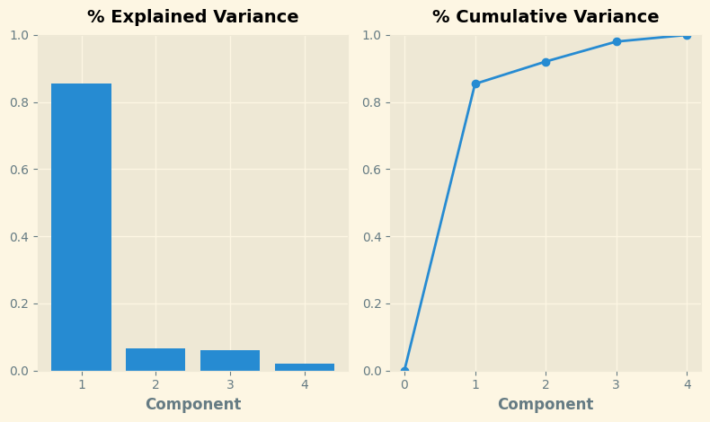

Let's also look at the MI scores of the components. Not surprisingly, PC1 is highly informative, though the remaining components, despite their small variance, still have a significant relationship with price. Examining those components could be worthwhile to find relationships not captured by the main Luxury/Economy axis.

我们还看一下组件的 MI 分数。 毫不奇怪，PC1信息量很大，而其余组件尽管差异很小，但仍然与价格有显著关系。 检查这些组成部分可能有助于发现主要豪华/经济轴未捕获的关系。

mi_scores = make_mi_scores(X_pca, y, discrete_features=False)
mi_scores

PC1    1.013262
PC2    0.379616
PC3    0.306072
PC4    0.204371
Name: MI Scores, dtype: float64

The third component shows a contrast between horsepower and curb_weight -- sports cars vs. wagons, it seems.

第三个组成部分显示了马力和整备重量之间的对比 —— 看起来是跑车与货车。

# Show dataframe sorted by PC3
idx = X_pca["PC3"].sort_values(ascending=False).index
cols = ["make", "body_style", "horsepower", "curb_weight"]
df.loc[idx, cols]

	make	body_style	horsepower	curb_weight
118	porsche	hardtop	207	2756
117	porsche	hardtop	207	2756
119	porsche	convertible	207	2800
45	jaguar	sedan	262	3950
96	nissan	hatchback	200	3139
...	...	...	...	...
59	mercedes-benz	wagon	123	3750
61	mercedes-benz	sedan	123	3770
101	peugot	wagon	95	3430
105	peugot	wagon	95	3485
143	toyota	wagon	62	3110

193 rows × 4 columns

To express this contrast, let's create a new ratio feature:

为了表达这种对比，让我们创建一个新的比率特征：

df["sports_or_wagon"] = X.curb_weight / X.horsepower
sns.regplot(x="sports_or_wagon", y='price', data=df, order=2);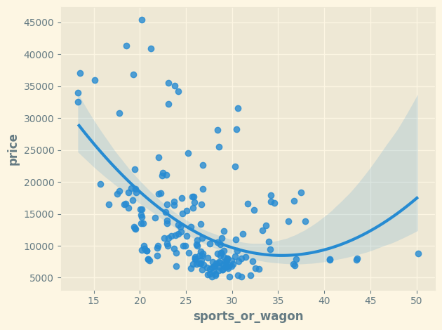

Your Turn

到你了

Improve your feature set by decomposing the variation in Ames Housing and use principal components to detect outliers.

通过分解 Ames Housing 中的变化改进您的特征集 并使用主成分来检测异常值。