Introduction

介绍

In the first two lessons, we learned how to build fully-connected networks out of stacks of dense layers. When first created, all of the network's weights are set randomly -- the network doesn't "know" anything yet. In this lesson we're going to see how to train a neural network; we're going to see how neural networks learn.

在前两课中，我们学习了如何用dense层的堆栈构建全连接的网络。 首次创建时，网络的所有权重都是随机设置的——网络还不知道任何事情。 在本课中，我们将了解如何训练神经网络； 我们将看到神经网络如何学习。

As with all machine learning tasks, we begin with a set of training data. Each example in the training data consists of some features (the inputs) together with an expected target (the output). Training the network means adjusting its weights in such a way that it can transform the features into the target. In the 80 Cereals dataset, for instance, we want a network that can take each cereal's 'sugar', 'fiber', and 'protein' content and produce a prediction for that cereal's 'calories'. If we can successfully train a network to do that, its weights must represent in some way the relationship between those features and that target as expressed in the training data.

与所有机器学习任务一样，我们从一组训练数据开始。 训练数据中的每个示例都包含一些特征（输入）和预期目标（输出）。 训练网络意味着调整其权重，使其能够将特征转化为目标。 例如，在 80 Cereals 数据集中，我们想要一个网络能够获取每种谷物的糖、纤维和蛋白质含量，并预测该谷物的卡路里 `。 如果我们能够成功地训练一个网络来做到这一点，它的权重必须以某种方式表示这些特征与训练数据中表达的目标之间的关系。

In addition to the training data, we need two more things:
除了训练数据之外，我们还需要两件事：

• A "loss function" that measures how good the network's predictions are.
• 衡量网络预测效果的损失函数。
• An "optimizer" that can tell the network how to change its weights.
• 一个优化器，可以告诉网络如何改变其权重。

The Loss Function

损失函数

We've seen how to design an architecture for a network, but we haven't seen how to tell a network what problem to solve. This is the job of the loss function.

我们已经了解了如何设计网络架构，但还没有了解如何告诉网络要解决什么问题。 这就是损失函数的工作。

The loss function measures the disparity between the the target's true value and the value the model predicts.

损失函数衡量目标真实值与模型预测值之间的差异。

Different problems call for different loss functions. We have been looking at regression problems, where the task is to predict some numerical value -- calories in 80 Cereals, rating in Red Wine Quality. Other regression tasks might be predicting the price of a house or the fuel efficiency of a car.

不同的问题需要不同的损失函数。 我们一直在研究回归问题，其中的任务是预测一些数值——80 种谷物中的卡路里，红酒质量中的评级。 其他回归任务可能是预测房屋的价格或汽车的燃油效率。

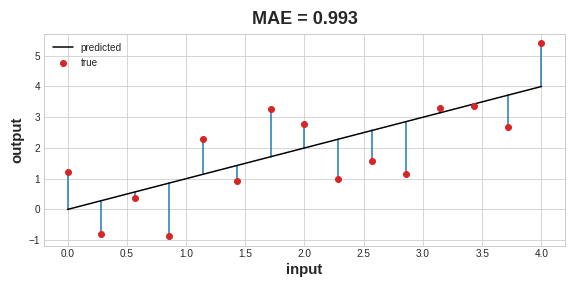
A common loss function for regression problems is the mean absolute error or MAE. For each prediction y_pred, MAE measures the disparity from the true target y_true by an absolute difference abs(y_true - y_pred).

回归问题的常见损失函数是平均绝对误差或MAE。 对于每个预测y_pred，MAE 通过绝对差abs(y_true - y_pred)来测量与真实目标y_true的差异。

The total MAE loss on a dataset is the mean of all these absolute differences.

数据集上的总 MAE 损失是所有这些绝对差值的平均值。

Besides MAE, other loss functions you might see for regression problems are the mean-squared error (MSE) or the Huber loss (both available in Keras).

除了 MAE 之外，您可能会在回归问题中看到的其他损失函数是均方误差 (MSE) 或 Huber 损失（两者都在 Keras 中可用）。

During training, the model will use the loss function as a guide for finding the correct values of its weights (lower loss is better). In other words, the loss function tells the network its objective.

在训练过程中，模型将使用损失函数作为寻找其权重的正确值的指南（损失越低越好）。 换句话说，损失函数告诉网络它的目标。

The Optimizer - Stochastic Gradient Descent

优化器 - 随机梯度下降

We've described the problem we want the network to solve, but now we need to say how to solve it. This is the job of the optimizer. The optimizer is an algorithm that adjusts the weights to minimize the loss.

我们已经描述了我们希望神经网络解决的问题，但现在我们需要说如何解决它。 这是优化器的工作。 优化器是一种调整权重以获得最小化损失的算法。

Virtually all of the optimization algorithms used in deep learning belong to a family called stochastic gradient descent. They are iterative algorithms that train a network in steps. One step of training goes like this:
事实上，深度学习中使用的所有优化算法都属于一个称为随机梯度下降的家族。 它们是逐步训练网络的迭代算法。 训练的一步是这样的：

1. Sample some training data and run it through the network to make predictions.
2. 对一些训练数据进行采样，并通过网络运行它来进行预测。
3. Measure the loss between the predictions and the true values.
4. 测量预测值与真实值之间的损失。
5. Finally, adjust the weights in a direction that makes the loss smaller.
6. 最后，向使损失变小的方向调整权重。

Then just do this over and over until the loss is as small as you like (or until it won't decrease any further.)

然后一遍又一遍地这样做，直到损失达到你想要的程度（或者直到它不再减少）。

Each iteration's sample of training data is called a minibatch (or often just "batch"), while a complete round of the training data is called an epoch. The number of epochs you train for is how many times the network will see each training example.

每次迭代的训练数据样本称为小批量（或通常只是批次），而完整一轮的训练数据称为纪元。 您训练的纪元数是网络将看到每个训练示例的次数。

The animation shows the linear model from Lesson 1 being trained with SGD. The pale red dots depict the entire training set, while the solid red dots are the minibatches. Every time SGD sees a new minibatch, it will shift the weights (w the slope and b the y-intercept) toward their correct values on that batch. Batch after batch, the line eventually converges to its best fit. You can see that the loss gets smaller as the weights get closer to their true values.

该动画显示了使用 SGD 训练第 1 课中的线性模型。 淡红点描绘了整个训练集，而实心红点是小批量。 每次 SGD 看到一个新的小批量时，它都会将权重（w斜率和b在 y 轴上的截距）移向该批次的正确值。 一批又一批，这条线最终收敛到最佳拟合。 您可以看到，随着权重越接近其真实值，损失就越小。

Learning Rate and Batch Size

学习率和批量大小

Notice that the line only makes a small shift in the direction of each batch (instead of moving all the way). The size of these shifts is determined by the learning rate. A smaller learning rate means the network needs to see more minibatches before its weights converge to their best values.

请注意，该线仅在每个批次的方向上进行小幅移动（而不是一路移动）。 这些变化的大小由学习率决定。 较小的学习率意味着网络在其权重收敛到最佳值之前需要使用更多的小批量。

The learning rate and the size of the minibatches are the two parameters that have the largest effect on how the SGD training proceeds. Their interaction is often subtle and the right choice for these parameters isn't always obvious. (We'll explore these effects in the exercise.)

学习率和小批量的大小是对 SGD 训练影响最大的两个参数。 它们的相互作用通常很微妙，并且这些参数的正确选择并不总是显而易见的。 （我们将在练习中探讨这些影响。）

Fortunately, for most work it won't be necessary to do an extensive hyperparameter search to get satisfactory results. Adam is an SGD algorithm that has an adaptive learning rate that makes it suitable for most problems without any parameter tuning (it is "self tuning", in a sense). Adam is a great general-purpose optimizer.

幸运的是，对于大多数工作来说，无需进行广泛的超参数搜索即可获得满意的结果。 Adam 是一种 SGD 算法，具有自适应学习率，使其适用于大多数问题，无需任何参数调整（从某种意义上来说，它是自调整）。 Adam 是一个出色的通用优化器。

Adding the Loss and Optimizer

添加损失和优化器

After defining a model, you can add a loss function and optimizer with the model's compile method:

定义模型后，您可以使用模型的compile方法添加损失函数和优化器：

model.compile(
    optimizer="adam",
    loss="mae",
)

Notice that we are able to specify the loss and optimizer with just a string. You can also access these directly through the Keras API -- if you wanted to tune parameters, for instance -- but for us, the defaults will work fine.

请注意，我们可以仅使用字符串来指定损失和优化器。 您还可以直接通过 Keras API 实现这些，—— 例如，如果您想调整参数 —— 但对我们来说，默认值就可以正常工作。

What's In a Name?
The gradient is a vector that tells us in what direction the weights need to go. More precisely, it tells us how to change the weights to make the loss change fastest. We call our process gradient descent because it uses the gradient to descend the loss curve towards a minimum. Stochastic means "determined by chance." Our training is stochastic because the minibatches are random samples from the dataset. And that's why it's called SGD!

名字有什么含义？
梯度是一个向量，告诉我们权重需要朝哪个方向移动。 更准确地说，它告诉我们如何改变权重以使损失变化最快。 我们将我们的过程称为梯度下降，因为它使用梯度将损失曲线下降到最小值。 随机的意思是“由机会决定”。 我们的训练是随机的，因为小批量是来自数据集的随机样本。 这就是为什么它被称为 SGD！

Example - Red Wine Quality

示例 - 红酒品质

Now we know everything we need to start training deep learning models. So let's see it in action! We'll use the Red Wine Quality dataset.

现在我们知道了开始训练深度学习模型所需的一切。 那么让我们来看看它的实际效果吧！ 我们将使用红酒质量数据集。

This dataset consists of physiochemical measurements from about 1600 Portuguese red wines. Also included is a quality rating for each wine from blind taste-tests. How well can we predict a wine's perceived quality from these measurements?

该数据集包含约 1600 种葡萄牙红酒的理化测量值。 还包括盲品测试中每种葡萄酒的质量评级。 我们如何通过这些测量来预测葡萄酒的感知质量？

We've put all of the data preparation into this next hidden cell. It's not essential to what follows so feel free to skip it. One thing you might note for now though is that we've rescaled each feature to lie in the interval $[0, 1]$. As we'll discuss more in Lesson 5, neural networks tend to perform best when their inputs are on a common scale.

我们已将所有数据准备工作放入下一个隐藏单元中。 这对于接下来的内容并不重要，所以可以跳过它。 不过，您现在可能会注意到的一件事是，我们已重新调整每个特征以使其位于区间 $[0, 1]$ 内。 正如我们将在第 5 课中详细讨论的那样，当神经网络的输入处于共同规模时，它们往往会表现最佳。

import pandas as pd
from IPython.display import display

red_wine = pd.read_csv('../00 datasets/ryanholbrook/dl-course-data/red-wine.csv')

# Create training and validation splits
df_train = red_wine.sample(frac=0.7, random_state=0)
df_valid = red_wine.drop(df_train.index)
display(df_train.head(4))

# Scale to [0, 1]
# 缩放至[0, 1]
max_ = df_train.max(axis=0)
min_ = df_train.min(axis=0)
df_train = (df_train - min_) / (max_ - min_)
df_valid = (df_valid - min_) / (max_ - min_)

# Split features and target
# 拆分特征与目标
X_train = df_train.drop('quality', axis=1)
X_valid = df_valid.drop('quality', axis=1)
y_train = df_train['quality']
y_valid = df_valid['quality']

	fixed acidity	volatile acidity	citric acid	residual sugar	chlorides	free sulfur dioxide	total sulfur dioxide	density	pH	sulphates	alcohol	quality
1109	10.8	0.470	0.43	2.10	0.171	27.0	66.0	0.99820	3.17	0.76	10.8	6
1032	8.1	0.820	0.00	4.10	0.095	5.0	14.0	0.99854	3.36	0.53	9.6	5
1002	9.1	0.290	0.33	2.05	0.063	13.0	27.0	0.99516	3.26	0.84	11.7	7
487	10.2	0.645	0.36	1.80	0.053	5.0	14.0	0.99820	3.17	0.42	10.0	6

How many inputs should this network have? We can discover this by looking at the number of columns in the data matrix. Be sure not to include the target ('quality') here -- only the input features.

该网络应该有多少个输入？ 我们可以通过查看数据矩阵中的列数来发现这一点。 确保这里不包含目标（质量）——仅包含输入特征。

print(X_train.shape)

(1119, 11)

Eleven columns means eleven inputs.

十一列意味着十一个输入。

We've chosen a three-layer network with over 1500 neurons. This network should be capable of learning fairly complex relationships in the data.

我们选择了一个包含超过 1500 个神经元的三层网络。 该网络应该能够学习数据中相当复杂的关系。

from tensorflow import keras
from tensorflow.keras import layers

model = keras.Sequential([
    layers.Dense(512, activation='relu', input_shape=[11]),
    layers.Dense(512, activation='relu'),
    layers.Dense(512, activation='relu'),
    layers.Dense(1),
])

2024-02-22 15:41:34.649841: I external/local_tsl/tsl/cuda/cudart_stub.cc:31] Could not find cuda drivers on your machine, GPU will not be used.
2024-02-22 15:41:37.715174: E external/local_xla/xla/stream_executor/cuda/cuda_dnn.cc:9261] Unable to register cuDNN factory: Attempting to register factory for plugin cuDNN when one has already been registered
2024-02-22 15:41:37.715250: E external/local_xla/xla/stream_executor/cuda/cuda_fft.cc:607] Unable to register cuFFT factory: Attempting to register factory for plugin cuFFT when one has already been registered
2024-02-22 15:41:37.731927: E external/local_xla/xla/stream_executor/cuda/cuda_blas.cc:1515] Unable to register cuBLAS factory: Attempting to register factory for plugin cuBLAS when one has already been registered
2024-02-22 15:41:37.774433: I external/local_tsl/tsl/cuda/cudart_stub.cc:31] Could not find cuda drivers on your machine, GPU will not be used.
2024-02-22 15:41:37.777150: I tensorflow/core/platform/cpu_feature_guard.cc:182] This TensorFlow binary is optimized to use available CPU instructions in performance-critical operations.
To enable the following instructions: AVX2 FMA, in other operations, rebuild TensorFlow with the appropriate compiler flags.
2024-02-22 15:41:40.957910: W tensorflow/compiler/tf2tensorrt/utils/py_utils.cc:38] TF-TRT Warning: Could not find TensorRT

Deciding the architecture of your model should be part of a process. Start simple and use the validation loss as your guide. You'll learn more about model development in the exercises.

决定模型的架构应该是这个过程的一部分。 从简单开始并使用验证损失作为指导。 您将在练习中了解有关模型开发的更多信息。

After defining the model, we compile in the optimizer and loss function.

定义模型后，我们编译优化器和损失函数。

model.compile(
    optimizer='adam',
    loss='mae',
)

Now we're ready to start the training! We've told Keras to feed the optimizer 256 rows of the training data at a time (the batch_size) and to do that 10 times all the way through the dataset (the epochs).

现在我们准备开始训练了！ 我们告诉 Keras 一次向优化器提供 256 行训练数据（batch_size），并在整个数据集（epochs）中执行 10 次。

history = model.fit(
    X_train, y_train,
    validation_data=(X_valid, y_valid),
    batch_size=256,
    epochs=10,
)

Epoch 1/10
5/5 [==============================] - 1s 66ms/step - loss: 0.2753 - val_loss: 0.1298
Epoch 2/10
5/5 [==============================] - 0s 25ms/step - loss: 0.1394 - val_loss: 0.1221
Epoch 3/10
5/5 [==============================] - 0s 27ms/step - loss: 0.1275 - val_loss: 0.1153
Epoch 4/10
5/5 [==============================] - 0s 27ms/step - loss: 0.1145 - val_loss: 0.1086
Epoch 5/10
5/5 [==============================] - 0s 30ms/step - loss: 0.1097 - val_loss: 0.1120
Epoch 6/10
5/5 [==============================] - 0s 30ms/step - loss: 0.1067 - val_loss: 0.1038
Epoch 7/10
5/5 [==============================] - 0s 31ms/step - loss: 0.1077 - val_loss: 0.1033
Epoch 8/10
5/5 [==============================] - 0s 28ms/step - loss: 0.1046 - val_loss: 0.1070
Epoch 9/10
5/5 [==============================] - 0s 24ms/step - loss: 0.1025 - val_loss: 0.1043
Epoch 10/10
5/5 [==============================] - 0s 31ms/step - loss: 0.1016 - val_loss: 0.0997

You can see that Keras will keep you updated on the loss as the model trains.

您可以看到 Keras 会在模型训练时向您报告损失的最新情况。

Often, a better way to view the loss though is to plot it. The fit method in fact keeps a record of the loss produced during training in a History object. We'll convert the data to a Pandas dataframe, which makes the plotting easy.

通常，查看损失的更好方法是将其绘制出来。 事实上，fit方法在History对象中保存了训练过程中产生的损失的记录。 我们将数据转换为 Pandas 数据框，这使得绘图变得容易。

import pandas as pd

# convert the training history to a dataframe
# 将训练历史数据转化为 DataFrame
history_df = pd.DataFrame(history.history)
# use Pandas native plot method
# 使用Pandas原生的plot方法
history_df['loss'].plot();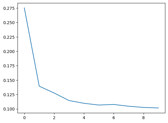

Notice how the loss levels off as the epochs go by. When the loss curve becomes horizontal like that, it means the model has learned all it can and there would be no reason continue for additional epochs.

请注意损失如何随着时间的增加而趋于平稳。 当损失曲线变得像这样水平时，这意味着模型已经学到了它能学到的一切，并且没有理由继续训练额外的纪元。

Your Turn

到你了

Now, use stochastic gradient descent to train your network.

现在，使用随机梯度下降 来训练您的网络。