This notebook is an exercise in the Intro to Deep Learning course. You can reference the tutorial at this link.

Introduction

介绍

In this exercise you'll train a neural network on the Fuel Economy dataset and then explore the effect of the learning rate and batch size on SGD.

在本练习中，您将在 Fuel Economy 数据集上训练神经网络，然后探索学习率和批量大小对 SGD 的影响。

When you're ready, run this next cell to set everything up!

准备好后，运行下一个单元格来设置一切！

# Setup plotting
import matplotlib.pyplot as plt
from learntools.deep_learning_intro.dltools import animate_sgd
plt.style.use('seaborn-v0_8-whitegrid')
# Set Matplotlib defaults
plt.rc('figure', autolayout=True)
plt.rc('axes', labelweight='bold', labelsize='large',
       titleweight='bold', titlesize=18, titlepad=10)
plt.rc('animation', html='html5')

# Setup feedback system
from learntools.core import binder
binder.bind(globals())
from learntools.deep_learning_intro.ex3 import *

2024-04-15 08:39:39.069831: E external/local_xla/xla/stream_executor/cuda/cuda_dnn.cc:9261] Unable to register cuDNN factory: Attempting to register factory for plugin cuDNN when one has already been registered
2024-04-15 08:39:39.069885: E external/local_xla/xla/stream_executor/cuda/cuda_fft.cc:607] Unable to register cuFFT factory: Attempting to register factory for plugin cuFFT when one has already been registered
2024-04-15 08:39:39.071449: E external/local_xla/xla/stream_executor/cuda/cuda_blas.cc:1515] Unable to register cuBLAS factory: Attempting to register factory for plugin cuBLAS when one has already been registered

In the Fuel Economy dataset your task is to predict the fuel economy of an automobile given features like its type of engine or the year it was made.

在Fuel Economy数据集中，您的任务是根据发动机类型或制造年份等特征来预测汽车的燃油经济性。

First load the dataset by running the cell below.

首先通过运行下面的单元格加载数据集。

import numpy as np
import pandas as pd
from sklearn.preprocessing import StandardScaler, OneHotEncoder
from sklearn.compose import make_column_transformer, make_column_selector
from sklearn.model_selection import train_test_split

fuel = pd.read_csv('../input/dl-course-data/fuel.csv')

X = fuel.copy()
# Remove target
y = X.pop('FE')

preprocessor = make_column_transformer(
    (StandardScaler(),
     make_column_selector(dtype_include=np.number)),
    (OneHotEncoder(sparse_output=False),
     make_column_selector(dtype_include=object)),
)

X = preprocessor.fit_transform(X)
y = np.log(y) # log transform target instead of standardizing

input_shape = [X.shape[1]]
print("Input shape: {}".format(input_shape))

Input shape: [50]

Take a look at the data if you like. Our target in this case is the 'FE' column and the remaining columns are the features.

如果你愿意的话可以看一下数据。在这种情况下，我们的目标是FE列，其余列是特征。

# Uncomment to see original data
fuel.head()
# Uncomment to see processed features
pd.DataFrame(X[:10,:]).head()

	0	1	2	3	4	5	6	7	8	...
0	0.913643	1.068005	0.524148	0.685653	-0.226455	0.391659	0.43492	0.463841	-0.447941	...
1	0.913643	1.068005	0.524148	0.685653	-0.226455	0.391659	0.43492	0.463841	-0.447941	...
2	0.530594	1.068005	0.524148	0.685653	-0.226455	0.391659	0.43492	0.463841	-0.447941	...
3	0.530594	1.068005	0.524148	0.685653	-0.226455	0.391659	0.43492	0.463841	-0.447941	...
4	1.296693	2.120794	0.524148	-1.458464	-0.226455	0.391659	0.43492	0.463841	-0.447941	...

5 rows × 50 columns

Run the next cell to define the network we'll use for this task.

运行下一个单元格来定义我们将用于此任务的网络。

from tensorflow import keras
from tensorflow.keras import layers

model = keras.Sequential([
    layers.Dense(128, activation='relu', input_shape=input_shape),
    layers.Dense(128, activation='relu'),    
    layers.Dense(64, activation='relu'),
    layers.Dense(1),
])

1) Add Loss and Optimizer

1) 添加损失和优化器

Before training the network we need to define the loss and optimizer we'll use. Using the model's compile method, add the Adam optimizer and MAE loss.

在训练网络之前，我们需要定义将使用的损失和优化器。使用模型的compile方法，添加 Adam 优化器和 MAE 损失。

# YOUR CODE HERE
# ____
model.compile(
    optimizer='adam',
    loss='mae',
)

# Check your answer
q_1.check()

Correct

# Lines below will give you a hint or solution code
#q_1.hint()
q_1.solution()

Solution:


model.compile(
    optimizer='adam',
    loss='mae'
)

2) Train Model

2) 训练模型

Once you've defined the model and compiled it with a loss and optimizer you're ready for training. Train the network for 200 epochs with a batch size of 128. The input data is X with target y.

一旦定义了模型并使用损失和优化器对其进行了编译，您就可以进行训练了。将网络训练 200 个 epoch，批量大小为 128。输入数据为X，目标为y。

# YOUR CODE HERE
# history = ____
history = model.fit(
    X, y,
    batch_size=128,
    epochs=200,
    verbose=False,
)

# Check your answer
q_2.check()

WARNING: All log messages before absl::InitializeLog() is called are written to STDERR
I0000 00:00:1713170384.452606     445 device_compiler.h:186] Compiled cluster using XLA!  This line is logged at most once for the lifetime of the process.

Correct

# Lines below will give you a hint or solution code
#q_2.hint()
q_2.solution()

Solution:


history = model.fit(
    X, y,
    batch_size=128,
    epochs=200
)

The last step is to look at the loss curves and evaluate the training. Run the cell below to get a plot of the training loss.

最后一步是查看损失曲线并评估训练。运行下面的单元格以获得训练损失图。

import pandas as pd

history_df = pd.DataFrame(history.history)
# Start the plot at epoch 5. You can change this to get a different view.
history_df.loc[5:, ['loss']].plot();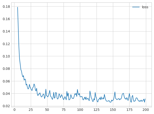

png

3) Evaluate Training

3) 评估训练

If you trained the model longer, would you expect the loss to decrease further?

如果你训练模型的时间更长，你会期望损失进一步减少吗？

# View the solution (Run this cell to receive credit!)
q_3.check()

Correct:

This depends on how the loss has evolved during training: if the learning curves have levelled off, there won't usually be any advantage to training for additional epochs. Conversely, if the loss appears to still be decreasing, then training for longer could be advantageous.

With the learning rate and the batch size, you have some control over:
通过学习率和批量大小，您可以控制：

How long it takes to train a model
训练模型需要多长时间
How noisy the learning curves are
学习曲线有多嘈杂
How small the loss becomes
损失有多小

To get a better understanding of these two parameters, we'll look at the linear model, our ppsimplest neural network. Having only a single weight and a bias, it's easier to see what effect a change of parameter has.

为了更好地理解这两个参数，我们将研究线性模型，即我们最简单的神经网络。只有单一权重和偏差，可以更容易地看出参数变化的影响。

The next cell will generate an animation like the one in the tutorial. Change the values for learning_rate, batch_size, and num_examples (how many data points) and then run the cell. (It may take a moment or two.) Try the following combinations, or try some of your own:

下一个单元格将生成类似于教程中的动画。更改learning_rate、batch_size和num_examples（多少个数据点）的值，然后运行单元。（可能需要一两分钟的时间。）尝试以下组合，或尝试您自己的组合：

`learning_rate`	`batch_size`	`num_examples`
0.05	32	256
0.05	2	256
0.05	128	256
0.02	32	256
0.2	32	256
1.0	32	256
0.9	4096	8192
0.99	4096	8192

# YOUR CODE HERE: Experiment with different values for the learning rate, batch size, and number of examples
learning_rate = [0.05, 0.05, 0.05]
batch_size = [32, 2, 128]
num_examples = [256, 256, 256]

# for i in range(1):
i=0
animate_sgd(
    learning_rate=learning_rate[i],
    batch_size=batch_size[i],
    num_examples=num_examples[i],
    # You can also change these, if you like
    steps=50, # total training steps (batches seen)
    true_w=3.0, # the slope of the data
    true_b=2.0, # the bias of the data
)
i=1
animate_sgd(
    learning_rate=learning_rate[i],
    batch_size=batch_size[i],
    num_examples=num_examples[i],
    # You can also change these, if you like
    steps=50, # total training steps (batches seen)
    true_w=3.0, # the slope of the data
    true_b=2.0, # the bias of the data
)

4) Learning Rate and Batch Size

4) 学习率和批量大小

What effect did changing these parameters have? After you've thought about it, run the cell below for some discussion.

改变这些参数有什么影响？在您考虑之后，请运行下面的单元格进行一些讨论。

# View the solution (Run this cell to receive credit!)
q_4.check()

Correct:

You probably saw that smaller batch sizes gave noisier weight updates and loss curves. This is because each batch is a small sample of data and smaller samples tend to give noisier estimates. Smaller batches can have an "averaging" effect though which can be beneficial.

Smaller learning rates make the updates smaller and the training takes longer to converge. Large learning rates can speed up training, but don't "settle in" to a minimum as well. When the learning rate is too large, the training can fail completely. (Try setting the learning rate to a large value like 0.99 to see this.)

Keep Going

继续前进

Learn how to improve your model's performance by tuning capacity or adding an early stopping callback.

了解如何通过调整容量或添加提前停止回调来提高模型的性能。

03.exercise-stochastic-gradient-descent【练习：随机梯度下降】