This notebook is an exercise in the Intro to Deep Learning course. You can reference the tutorial at this link.

Introduction

介绍

In this exercise, you'll add dropout to the Spotify model from Exercise 4 and see how batch normalization can let you successfully train models on difficult datasets.

在本练习中，您将向练习 4 中的 Spotify 模型添加 dropout，并了解批量归一化如何让您在困难的数据集上成功训练模型。

Run the next cell to get started!

运行下一个单元格即可开始！

# Setup plotting
import matplotlib.pyplot as plt
plt.style.use('seaborn-v0_8-whitegrid')
# Set Matplotlib defaults
plt.rc('figure', autolayout=True)
plt.rc('axes', labelweight='bold', labelsize='large',
       titleweight='bold', titlesize=18, titlepad=10)
plt.rc('animation', html='html5')

# Setup feedback system
from learntools.core import binder
binder.bind(globals())
from learntools.deep_learning_intro.ex5 import *

First load the Spotify dataset.

首先加载 Spotify 数据集。

import pandas as pd
from sklearn.preprocessing import StandardScaler, OneHotEncoder
from sklearn.compose import make_column_transformer
from sklearn.model_selection import GroupShuffleSplit

from tensorflow import keras
from tensorflow.keras import layers
from tensorflow.keras import callbacks

spotify = pd.read_csv('../input/dl-course-data/spotify.csv')

X = spotify.copy().dropna()
y = X.pop('track_popularity')
artists = X['track_artist']

features_num = ['danceability', 'energy', 'key', 'loudness', 'mode',
                'speechiness', 'acousticness', 'instrumentalness',
                'liveness', 'valence', 'tempo', 'duration_ms']
features_cat = ['playlist_genre']

preprocessor = make_column_transformer(
    (StandardScaler(), features_num),
    (OneHotEncoder(), features_cat),
)

def group_split(X, y, group, train_size=0.75):
    splitter = GroupShuffleSplit(train_size=train_size)
    train, test = next(splitter.split(X, y, groups=group))
    return (X.iloc[train], X.iloc[test], y.iloc[train], y.iloc[test])

X_train, X_valid, y_train, y_valid = group_split(X, y, artists)

X_train = preprocessor.fit_transform(X_train)
X_valid = preprocessor.transform(X_valid)
y_train = y_train / 100
y_valid = y_valid / 100

input_shape = [X_train.shape[1]]
print("Input shape: {}".format(input_shape))

2024-04-25 06:06:56.524549: E external/local_xla/xla/stream_executor/cuda/cuda_dnn.cc:9261] Unable to register cuDNN factory: Attempting to register factory for plugin cuDNN when one has already been registered
2024-04-25 06:06:56.524599: E external/local_xla/xla/stream_executor/cuda/cuda_fft.cc:607] Unable to register cuFFT factory: Attempting to register factory for plugin cuFFT when one has already been registered
2024-04-25 06:06:56.526029: E external/local_xla/xla/stream_executor/cuda/cuda_blas.cc:1515] Unable to register cuBLAS factory: Attempting to register factory for plugin cuBLAS when one has already been registered

Input shape: [18]

1) Add Dropout to Spotify Model

1) 将 Dropout 层添加到 Spotify 模型

Here is the last model from Exercise 4. Add two dropout layers, one after the Dense layer with 128 units, and one after the Dense layer with 64 units. Set the dropout rate on both to 0.3.

这是练习 4 中的最后一个模型。添加两个 dropout 层，一个位于具有 128 个单元的Dense层之后，另一个位于具有 64 个单元的Dense层之后。将两者的退出率设置为0.3。

# YOUR CODE HERE: Add two 30% dropout layers, one after 128 and one after 64
model = keras.Sequential([
    layers.Dense(128, activation='relu', input_shape=input_shape),
    layers.Dropout(rate=0.3),
    layers.Dense(64, activation='relu'),
    layers.Dropout(rate=0.3),
    layers.Dense(1)
])

# Check your answer
q_1.check()

Correct

# Lines below will give you a hint or solution code
#q_1.hint()
q_1.solution()

Solution:


model = keras.Sequential([
    layers.Dense(128, activation='relu', input_shape=input_shape),
    layers.Dropout(0.3),
    layers.Dense(64, activation='relu'),
    layers.Dropout(0.3),
    layers.Dense(1)
])

Now run this next cell to train the model see the effect of adding dropout.

现在运行下一个单元格来训练模型，看看添加 dropout 的效果。

model.compile(
    optimizer='adam',
    loss='mae',
)
history = model.fit(
    X_train, y_train,
    validation_data=(X_valid, y_valid),
    batch_size=512,
    epochs=50,
    verbose=0,
)
history_df = pd.DataFrame(history.history)
history_df.loc[:, ['loss', 'val_loss']].plot()
print("Minimum Validation Loss: {:0.4f}".format(history_df['val_loss'].min()))

WARNING: All log messages before absl::InitializeLog() is called are written to STDERR
I0000 00:00:1714025222.439856    2374 device_compiler.h:186] Compiled cluster using XLA!  This line is logged at most once for the lifetime of the process.

Minimum Validation Loss: 0.1954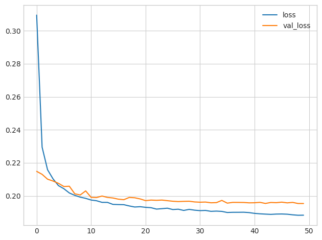

png

2) Evaluate Dropout

2) 评估 Dropout

Recall from Exercise 4 that this model tended to overfit the data around epoch 5. Did adding dropout seem to help prevent overfitting this time?

回想一下练习 4，该模型在 epoch 5 附近开始倾向于过度拟合数据。这次添加 dropout 似乎有助于防止过度拟合吗？

# View the solution (Run this cell to receive credit!)
q_2.check()

Correct:

From the learning curves, you can see that the validation loss remains near a constant minimum even though the training loss continues to decrease. So we can see that adding dropout did prevent overfitting this time. Moreover, by making it harder for the network to fit spurious patterns, dropout may have encouraged the network to seek out more of the true patterns, possibly improving the validation loss some as well).

从学习曲线中，您可以看到，即使训练损失持续减少，验证损失仍保持在恒定的最小值附近。所以我们可以看到，这次添加dropout确实防止了过拟合。此外，通过使网络更难适应虚假模式，dropout 可能会鼓励网络寻找更多真实模式，也可能改善验证损失。

Now, we'll switch topics to explore how batch normalization can fix problems in training.

现在，我们将转换主题来探讨批量归一化如何解决训练中的问题。

Load the Concrete dataset. We won't do any standardization this time. This will make the effect of batch normalization much more apparent.

加载水泥数据集。这次我们不会做任何标准化。这将使批量归一化的效果更加明显。

import pandas as pd

concrete = pd.read_csv('../input/dl-course-data/concrete.csv')
df = concrete.copy()

df_train = df.sample(frac=0.7, random_state=0)
df_valid = df.drop(df_train.index)

X_train = df_train.drop('CompressiveStrength', axis=1)
X_valid = df_valid.drop('CompressiveStrength', axis=1)
y_train = df_train['CompressiveStrength']
y_valid = df_valid['CompressiveStrength']

input_shape = [X_train.shape[1]]

Run the following cell to train the network on the unstandardized Concrete data.

运行以下单元以使用非归一化的水泥数据训练网络。

model = keras.Sequential([
    layers.Dense(512, activation='relu', input_shape=input_shape),
    layers.Dense(512, activation='relu'),    
    layers.Dense(512, activation='relu'),
    layers.Dense(1),
])
model.compile(
    optimizer='sgd', # SGD is more sensitive to differences of scale
    loss='mae',
    metrics=['mae'],
)
history = model.fit(
    X_train, y_train,
    validation_data=(X_valid, y_valid),
    batch_size=64,
    epochs=100,
    verbose=0,
)

history_df = pd.DataFrame(history.history)
history_df.loc[0:, ['loss', 'val_loss']].plot()
print(("Minimum Validation Loss: {:0.4f}").format(history_df['val_loss'].min()))

Minimum Validation Loss: nan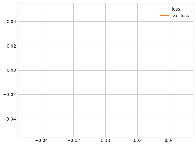

png

Did you end up with a blank graph? Trying to train this network on this dataset will usually fail. Even when it does converge (due to a lucky weight initialization), it tends to converge to a very large number.

您最终得到的是空白图表吗？尝试在此数据集上训练该网络通常会失败。即使它确实收敛（由于幸运的权重初始化），它也往往会收敛到一个非常大的数字。

3) Add Batch Normalization Layers

3) 添加批量归一化层

Batch normalization can help correct problems like this.

批量归一化可以帮助纠正此类问题。

Add four BatchNormalization layers, one before each of the dense layers. (Remember to move the input_shape argument to the new first layer.)

添加四个BatchNormalization层，每个密集层之前都有一个。（记住将input_shape参数移至新的第一层。）

# YOUR CODE HERE: Add a BatchNormalization layer before each Dense layer
# model = keras.Sequential([
#     layers.Dense(512, activation='relu', input_shape=input_shape),
#     layers.Dense(512, activation='relu'),
#     layers.Dense(512, activation='relu'),
#     layers.Dense(1),
# ])

model = keras.Sequential([
    layers.BatchNormalization(input_shape=input_shape),
    layers.Dense(512, activation='relu'),
    layers.BatchNormalization(),
    layers.Dense(512, activation='relu'),
    layers.BatchNormalization(),
    layers.Dense(512, activation='relu'),
    layers.BatchNormalization(),
    layers.Dense(1),
])

# Check your answer
q_3.check()

Correct

# Lines below will give you a hint or solution code
#q_3.hint()
q_3.solution()

Solution:


model = keras.Sequential([
    layers.BatchNormalization(input_shape=input_shape),
    layers.Dense(512, activation='relu'),
    layers.BatchNormalization(),
    layers.Dense(512, activation='relu'),
    layers.BatchNormalization(),
    layers.Dense(512, activation='relu'),
    layers.BatchNormalization(),
    layers.Dense(1),
])

Run the next cell to see if batch normalization will let us train the model.

运行下一个单元格，看看批量归一化是否能让我们训练模型。

model.compile(
    optimizer='sgd',
    loss='mae',
    metrics=['mae'],
)
EPOCHS = 100
history = model.fit(
    X_train, y_train,
    validation_data=(X_valid, y_valid),
    batch_size=64,
    epochs=EPOCHS,
    verbose=0,
)

history_df = pd.DataFrame(history.history)
history_df.loc[0:, ['loss', 'val_loss']].plot()
print(("Minimum Validation Loss: {:0.4f}").format(history_df['val_loss'].min()))

Minimum Validation Loss: 3.7829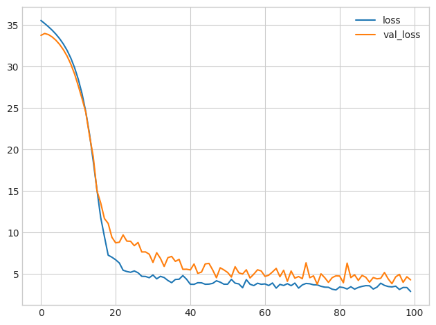

png

4) Evaluate Batch Normalization

4) 评估批量归一化

Did adding batch normalization help?

添加批量归一化有帮助吗？

# View the solution (Run this cell to receive credit!)
q_4.check()

Correct:

You can see that adding batch normalization was a big improvement on the first attempt! By adaptively scaling the data as it passes through the network, batch normalization can let you train models on difficult datasets.

您可以看到，添加批量归一化比第一次尝试有了很大的进步！通过在数据通过网络时自适应地缩放数据，批量归一化可以让您在困难的数据集上训练模型。

Keep Going

继续前进

Create neural networks for binary classification.

创建神经网络进行二元分类。

05.exercise-dropout-and-batch-normalization【练习：暂退层及批量归一化】